Checking the friction law in simple shear
Before you trust an earthquake-cycle model, check that DES reproduces the friction law itself. This benchmark shears a single square cell at a known rate. With every node velocity prescribed, there is no wave, localization or mesh effect, so the stress, friction and state can be compared directly with closed-form solutions. It runs in about half a minute.
The benchmark covers four groups:
| Group | Cases | Varied |
|---|---|---|
| Elastoplastic (static friction) | 3 | friction angle 10°, 20°, 30° |
Steady-state RSF (state_var_model = 0) | 3 | m/s |
Aging-law RSF (state_var_model = 1) | 3 | m |
| Healing at zero slip rate | 1 | – |
See rate-and-state friction for the equations used below.
| Dimension | 2D |
| Build | make ndims=2 |
| Run time | about 30 s for all cases, one thread |
| Inputs | benchmarks/faults-friction/simple_shear_rsf/ in the DynEarthSol repository |
| Checked with | DynEarthSol 68cc2a0 |
Setup
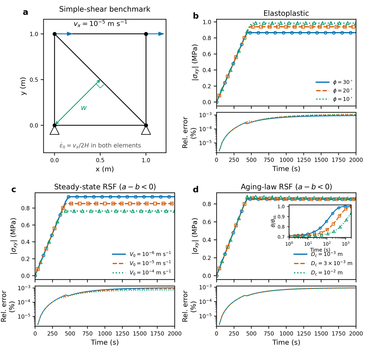
Figure 1. (a) The cell: two triangles in a 1 m square. The bottom nodes are fixed and the top nodes move at m/s. (b–d) Shear stress from DES (lines) and the reference (markers), with the relative error below each panel. The inset in (d) shows the state variable relative to its steady-state value.
| Setting | Value |
|---|---|
| Cell | 1 m × 1 m, two triangles, plane strain |
| Loading | top moves at m/s; bottom fixed |
| Bulk and shear moduli | 200 MPa and 200 MPa |
| Cohesion | 1 MPa, no weakening; zero dilation; no gravity |
| RSF parameters | , , |
| Slip-rate measure | strain-rate invariant (control.rsf_slip_rate_projection_option = 1) |
| Time step | fixed, 0.01 s, 200,000 steps (2000 s, shear strain 0.02) |
The large and make the differences between cases easy to see. The cell deforms isochorically and without gravity, so the mean stress stays zero and the Mohr–Coulomb shear strength is with .
Reference solutions
Stress. The cell loads elastically and then flows at its strength:
with for the elastoplastic cases and the RSF friction coefficient otherwise.
Slip rate. In the shearing two-triangle cell the strain-rate measure gives
because the element width changes as the cell shears.
Steady state. at the current .
Aging law. With , the aging law has the solution
which the reference evaluates by quadrature. The friction follows from the full law.
Healing. A separate run holds the cell still for 1546 steps of three days ( m, m/s). The slip rate is then the m/s floor and the state grows almost linearly with time, . The check iterates DES's discrete update independently.
Input and how to run
Build dynearthsol2d in the DES root, then:
cd benchmarks/faults-friction/simple_shear_rsf
python3 run_simple_shear_benchmark.py --clean --aging-transient --healing
python3 plot_simple_shear_benchmark.py -o simple_shear_benchmark.png
The runner writes one input file per case from simple_shear_base.cfg,
which holds placeholders for the values in the table above, and runs DES in
runs/<case>/. --aging-transient adds three runs with dense monitor output
for the inset in panel (d); --healing adds the zero-velocity run. Pass
--exe /path/to/dynearthsol2d if the executable is elsewhere.
For a pass/fail check without plotting:
python3 check_simple_shear_benchmark.py          # one steady, one aging, healing
python3 check_simple_shear_benchmark.py --all    # all nine cases and healing
Add --pt to run the same cases with PT mechanics.
The key RSF lines in a generated input are:
[control]
use_global_velocity_scaling = true
rsf_slip_rate_projection_option = 1
fixed_dt = 0.01

[mat]
rheology_type = elasto-plastic-rate-state-friction
direct_a = [0.2]
evolution_b = [0.3]
characteristic_velocity = [1e-05]
characteristic_distance = [0.001]
state_var_model = 1

[monitor]
enabled = yes
num_points = 2
output_stress = yes
output_dynamic_friction = yes
output_state_variable = yes
Output
Each runs/<case>/ holds the input, the DES output and two monitor files,
monitor_point_0.csv and monitor_point_1.csv, one per element. Their
columns include stress_0, stress_1, stress_2 (σxx, σzz, σxz),
dynamic_friction and state_variable. The plot script compares the mean
absolute shear stress of the two elements with the reference and writes
simple_shear_benchmark_metrics.csv.
Result
In every case DES follows the reference through loading, yield and flow. The largest difference over the run is about 0.001 % of the reference stress:
| Case | Maximum error (%) |
|---|---|
| Elastoplastic, φ = 30°, 20°, 10° | 0.00091, 0.00106, 0.00116 |
| Steady state, = 10⁻⁶, 10⁻⁵, 10⁻⁴ m/s | 0.00105, 0.00089, 0.00072 |
| Aging law, = 10⁻³, 3×10⁻³, 10⁻² m | 0.00089, 0.00089, 0.00091 |
The checker also recovers the slip rate DES used from the monitored friction and state; it matches to a relative error of . The healing run matches the discrete update exactly.
Things to notice in the figure:
- Panel (b). A lower friction angle gives a higher strength here, because at zero mean stress. Friction only adds strength through normal stress, and this cell has none.
- Panel (c). With , a larger means the cell slides slower relative to the reference rate, so the friction is higher and the strength lower.
- Panel (d). All three values reach nearly the same stress, but the state approaches steady state more slowly for larger (inset): the slip needed to renew the contacts is larger.
Limits
This benchmark checks the constitutive update in a homogeneous cell with prescribed motion. It does not test localization, wave propagation, mesh dependence or the coupling between slip and elastic unloading that controls earthquake nucleation. Under PT, the prescribed motion balances the forces at the first iteration, so the PT run checks the accepted constitutive history, not iterative convergence. The earthquake-cycle tutorial adds those effects.