Shear bands with and without rate-and-state friction
A brittle crust pulled apart from a weak seed localizes into shear bands.
This benchmark runs the same model three times, with static Mohr–Coulomb
friction (EP) and with rate-and-state friction that is velocity
strengthening or velocity weakening (EP-RSF). It asks two questions: does
rate-and-state friction change where and at what angle the bands form, and
does it change how they slip? The inputs are the DES v2 benchmark in
benchmarks/geodynamics/localization/; see
rate-and-state friction for the
friction law and for global velocity scaling.
| Dimension | 2D |
| Build | make ndims=2 |
| Run time | 35 minutes (EP), 75 minutes (weakening) and 3 hours (strengthening) on 8 threads |
| Inputs | benchmarks/geodynamics/localization/ in the DynEarthSol repository |
| Results | the benchmark results given in its README |
Setup
| Setting | Value |
|---|---|
| Domain | 20 km × 10 km, uniform triangles of 100 m (meshing_option = 1) |
| Loading | both sides pulled outward at 0.5 cm/yr each; free top; Winkler support at the base; gravity 10 m/s² |
| Initial state | lithostatic stress; a circular seed of radius 500 m centred at (10, −9.5) km starts with plastic strain 1 |
| Elasticity and density | = 50 GPa, = 30 GPa, 2700 kg/m³ |
| Strength | friction angle 30°, no dilation; cohesion softening from 30 to 0.1 MPa over plastic strain 0 to 0.5 |
| Rate-and-state | aging law, = 5 mm, m/s, strain-rate slip measure (rsf_slip_rate_projection_option = 1), state limit rsf_dtheta_max = 0.2 |
| Mechanics | explicit, global velocity scaling with , damping factor 0.8 |
| Duration | 12,000 years, a frame every 500 years |
The three inputs differ only in the friction law:
| Input | Rheology | |||
|---|---|---|---|---|
ep_phi30_psi0.cfg | elasto-plastic | – | – | – |
ep_rsf_strengthening_phi30_psi0.cfg | elasto-plastic-rsf | 0.018 | 0.015 | 1.2 |
ep_rsf_weakening_phi30_psi0.cfg | elasto-plastic-rsf | 0.003 | 0.015 | 0.2 |
For a Mohr–Coulomb material with friction angle and dilation angle , the Arthur angle predicts bands at from the direction of the least compressive stress, here from the horizontal.
Input and how to run
Build dynearthsol2d in the DES root, then run each input from the
benchmark folder:
cd benchmarks/geodynamics/localization
mkdir -p output
OMP_NUM_THREADS=8 ../../../dynearthsol2d ep_phi30_psi0.cfg
OMP_NUM_THREADS=8 ../../../dynearthsol2d ep_rsf_strengthening_phi30_psi0.cfg
OMP_NUM_THREADS=8 ../../../dynearthsol2d ep_rsf_weakening_phi30_psi0.cfg
Each writes to output/ under its own name: frames <name>.save.*,
checkpoints, <name>.info, and three monitor files,
<name>_monitor_point_0.csv to _2.csv, recorded every 1000 steps. Point 1
starts at the seed centre; points 0 and 2 lie near the side walls.
What to look for
Where the bands form
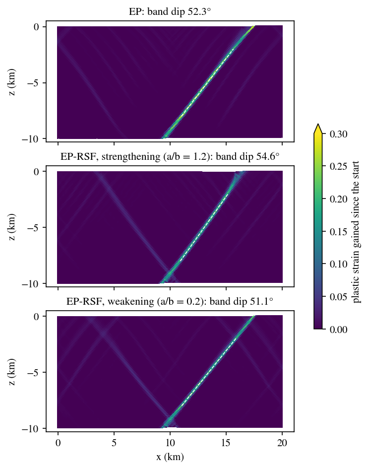
All three models break the crust along a band that rises from the seed to the surface on the right, with a fainter conjugate band on the left. The band carries most of the extension; the rest of the crust stays elastic.
| Model | Band dip (fit over 2–8 km) |
|---|---|
| EP | 52.4° |
| EP-RSF, strengthening | 54.5° |
| EP-RSF, weakening | 51.2° |
| Arthur angle, | 52.5° |
Rate-and-state friction moves the dip by about two degrees at most. The orientation is set by the Mohr–Coulomb strength, not by the rate dependence. Velocity strengthening steepens the band slightly; velocity weakening flattens it slightly.
The dip is measured from the plastic strain gained since frame 0, so the initial seed does not count. In each 200 m depth row between 2 and 8 km, take the element with the largest gain on each side of the seed, keep it if the gain exceeds a quarter of the maximum, and fit a straight line through the points:
import numpy as np
from Dynearthsol import Dynearthsol

des = Dynearthsol('output/ep_phi30_psi0')
first, last = des.frames[0], des.frames[-1]
x = des.read_field(last, 'coordinate')/1e3          # km
c = des.read_field(last, 'connectivity')
gain = des.read_field(last, 'plastic strain') - des.read_field(first, 'plastic strain')
cen = x[c].mean(axis=1)
zs, xs = [], []
for z0 in np.arange(-8.0, -2.0, 0.2):
    row = (cen[:, 0] >= 10) & (cen[:, 1] >= z0) & (cen[:, 1] < z0 + 0.2)
    i = np.argmax(np.where(row, gain, -np.inf))
    if gain[i] > 0.25*gain.max():
        zs.append(cen[i, 1]); xs.append(cen[i, 0])
slope = np.polyfit(zs, xs, 1)[0]
print('dip', np.degrees(np.arctan(1/abs(slope))))
Run it from the benchmark folder with the DES root on PYTHONPATH. It gives
the dips in the table to within 0.1°. Use cen[:, 0] < 10 for the band on
the left; in these runs only the right band passes the threshold over the
whole depth range.
How the bands slip
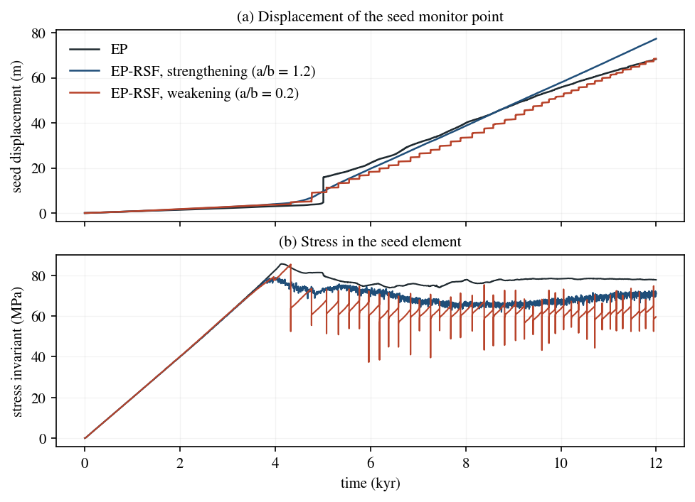
The monitor at the seed (_monitor_point_1.csv) shows three different
ways of slipping on almost the same band. The stress invariant is
sqrt(0.25*(stress_0 - stress_1)**2 + stress_2**2) of the seed element.
- Loading is the same in all three. The stress rises linearly for about 4000 years while the crust deforms elastically.
- EP fails once, then slides. The stress peaks at 86 MPa at 4.1 kyr. At 5.0 kyr the band breaks through to the surface in one fast slip: the seed moves about 12 m at up to 5 cm/s. After that the band slides steadily at about 78 MPa.
- Velocity strengthening creeps. The stress peaks lower, at 79 MPa at
4.0 kyr, and the band then slides steadily at about 68 MPa. The seed never
exceeds 1 cm/s and there are no slip events. The friction coefficient in
the seed element (
dynamic_friction) varies between about 0.54 and 0.81 from one monitor row to the next. - Velocity weakening sticks and slips. The stress reaches 85 MPa before the first event at 4.3 kyr. Then 39 events follow until 12 kyr. The gap between events shortens from about 440 years to about 180 years after 8 kyr. In a typical event the seed slips 1.3 m (0.5 to 2.0 m) in about a minute at 0.1 to 0.8 m/s, and the stress in the seed element drops by 5 MPa (up to 21 MPa). Most events are followed a few years later by a slow slip of about 0.3 m with no stress drop. Between events the stress recovers along a straight line, as in the loading phase.
The boundaries pull at the same rate in all three, and the seed has moved 68 to 77 m by 12 kyr in each. What differs is when that slip happens. Global velocity scaling lets one run carry both the centuries between events and the seconds of each event: the time step falls from about s between events to below s during them.
Limits
- One element. The stress and friction histories come from the seed element and the displacement from one node. They show the character of slip, not the slip distribution along the band.
- One resolution. All runs use 100 m elements, so the band is a few elements wide. The dips have not been checked at other resolutions.
- One band. Only the band on the right is clear enough to fit over 2–8 km. The conjugate band is weaker in all three models.
Exercises
- Change the dilation angle. Set
dilation_angle0anddilation_angle1to 15 and compare the dips with the Arthur angle, now 56.25°. - Move through 1. Run = 0.012, 0.015 and 0.016 with = 0.015 and find where the slip events stop.
- Count the events. With
sim.seismic_moment_calculate_output = yesthe weakening case writes each event's moment toseismic_moment_magnitude.txt. Compare it with the seed slip in the monitor file.