Elastic loading and equilibrium
This exercise compresses a 1 m elastic cell with a constant top traction. You will run both pseudo-transient schemes, compare the result with an analytical elastic response, and see why a held load does not produce repeated compression. Finish by restarting from a held state and applying a larger load.
| Dimension | 2D (a 3D variant is described at the end) |
| Build | make ndims=2 hdf5=0 |
| Run time | under a second per case, one thread |
| Inputs | the PT tutorial bundle (elastic-0.cfg, elastic-1.cfg, analyze_pt.py) |
| Checked with | figures from DynEarthSol 707e481; reproduced on 68cc2a0 |
Build the checked solver
Use a new terminal and a separate checkout. You need Git, Make, a C++17
compiler, and Python 3. On Debian/Ubuntu, install git g++ make python3 python3-venv; on macOS, install the Xcode Command Line Tools and Homebrew's
libomp and python. See installation for other platforms.
The config parser is bundled with the source.
git clone https://github.com/GeoFLAC/DynEarthSol.git DynEarthSol-pt-tutorial
cd DynEarthSol-pt-tutorial
make -j2 ndims=2 hdf5=0
./dynearthsol2d --help
make fetches the required nanoflann submodule. This exercise needs no
MMG, Exodus, GPU or HDF5 build. Confirm that help includes PT_option,
PT_use_running_scale and PT_absolute_tolerance.
Prepare Python in the same checkout:
python3 -m venv .venv
source .venv/bin/activate
python -m pip install numpy matplotlib
export OMP_NUM_THREADS=1
export OMP_DYNAMIC=FALSE
Get the tutorial inputs
Download the tutorial bundle and extract it
into a new pt-tutorial directory inside the solver checkout. The bundle
contains the four elastic/Maxwell configs, analyze_pt.py, and a README.
From the checkout root, the equivalent terminal commands are:
python - <<'PY'
from pathlib import Path
from urllib.request import urlretrieve
from zipfile import ZipFile

destination = Path("pt-tutorial")
destination.mkdir()  # Use a new directory for a fresh exercise.
urlretrieve("https://geoflac.github.io/des3d/tutorial/pt/pt-tutorial.zip",
            destination / "pt-tutorial.zip")
with ZipFile(destination / "pt-tutorial.zip") as archive:
    archive.extractall(destination)
PY
cd pt-tutorial
You can also inspect option 0,
option 1 and the
analysis script individually. The elastic
configs reproduce the upstream examples/fundamentals/pt-elastic-load.cfg with distinct
output names and the selected PT_option.
Geometry and loading
The 2D domain spans m and m. The sides are horizontal rollers: horizontal velocity is zero, and vertical motion is free. The base is clamped. The top is free in velocity and carries a vertical traction of kPa. Compression is negative in DES output.
| Setting | Value |
|---|---|
| Bulk modulus / shear modulus | 10 MPa / 10 MPa |
| Gravity / hydraulic diffusion / surface processes | Disabled |
| Nominal resolution | 0.5 m |
| Physical timestep / duration | 0.01 s / 3 steps |
| Mesh motion / remeshing | Disabled |
| Field and checkpoint output | Every physical step, without time averaging |
| PT convergence mode | PT_use_running_scale = yes |
The important controls in both configs are:
[control]
has_PT = yes
PT_option = 0
PT_max_iter = 5000
PT_use_running_scale = yes
fixed_dt = 0.01
has_moving_mesh = no
has_hydraulic_diffusion = no
gravity = 0
surface_process_option = 0
elastic-1.cfg changes PT_option to 1 and the output name to
elastic-1. The running scale keeps force precision tied to the applied
load during subsequent held steps. It is an explicit tutorial setting;
the solver default is no. Read its
scope and limitations before using
it in another problem.
Run and plot
From DynEarthSol-pt-tutorial/pt-tutorial, run:
../dynearthsol2d elastic-0.cfg > elastic-0.log 2>&1
../dynearthsol2d elastic-1.cfg > elastic-1.log 2>&1
python analyze_pt.py elastic elastic-0 elastic-1 --source ..
Each model writes a .info index, a .manifest, and save/checkpoint
frames 0 through 3. The script reads the native output through the
checkout's Dynearthsol.py. It checks all components of saved stress,
strain, coordinates and velocity for finiteness, then compares axial stress,
axial strain and vertical velocity against the homogeneous reference and
checks convergence records. It writes elastic-0.csv, elastic-1.csv,
elastic-response.svg/.png and elastic-convergence.svg/.png.
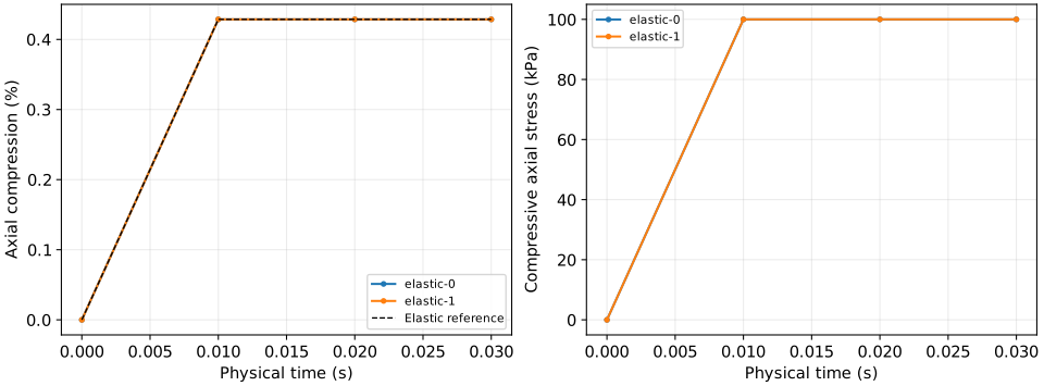
For the laterally confined response,
After the first physical step, expect approximately kPa vertical stress and vertical strain. Steps 2 and 3 retain that compression. Both schemes should agree with this response within the solver tolerance; the checked runs have normalized field errors below . The analysis script uses a acceptance limit, normalizing stress by 100 kPa, strain by 0.01, and velocity by 0.5 m/s.
Because mesh motion is disabled, the coordinates remain unchanged. The equivalent top displacement is reconstructed as , approximately −4.286 mm. This deliberately fixed-grid constitutive exercise is not a moving-boundary compression experiment.
Interpret the convergence records
rg '^PT step=' elastic-0.log elastic-1.log
Use grep '^PT step=' elastic-0.log elastic-1.log if ripgrep is unavailable.
The checked serial runs give:
| Physical step | Option 0 iterations / evaluations | Option 1 iterations / evaluations |
|---|---|---|
| 1: apply the load | 299 / 299 | 25 / 25 |
| 2: hold the load | 1 / 2 | 1 / 2 |
| 3: hold the load | 1 / 1 | 1 / 1 |
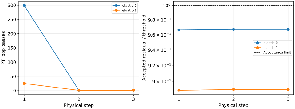
Iteration counts can vary with platform and compiler. In both options, the first step needs relaxation. Step 2 compares the old loading velocity with zero free motion; the latter already meets the threshold. Step 3 starts from the retained zero velocity. One loop pass therefore means no relaxation update, while two evaluations mean two full candidates were checked.
The 2D option-0 step-1 residual is about 0.0341744 N/m and its threshold
is 0.0353553 N/m. The residual is a projected nodal-force RMS, not a stress
in Pa. initial describes the selected candidate; warm_initial can be
much larger after the candidate comparison. All records state
stage=before_physical_updates.
For physical steps, this label follows any thermal diffusion update and
precedes hydraulic transport, mesh motion and stress rotation.
The saved PT residual force has this same diagnostic time level. Saved
stress includes the later physical stress rotation, so independently
assembling force from it need not reproduce exactly the printed residual.
See the force-output reference.
Restart and double the load
This Python block copies the option-0 config into a new restart config,
selects the checkpoint at frame 2, and doubles the top traction. Run it
in the same pt-tutorial directory:
python - <<'PY'
import configparser

cfg = configparser.ConfigParser()
cfg.optionxform = str
cfg.read("elastic-0.cfg")
cfg["sim"].update(modelname="elastic-reload", is_restarting="yes",
                  restarting_from_modelname="elastic-0",
                  restarting_from_frame="2")
cfg["bc"]["stress_val_z1"] = "-2e5"
with open("elastic-reload.cfg", "w") as stream:
    cfg.write(stream)
PY
../dynearthsol2d elastic-reload.cfg > elastic-reload.log 2>&1
python - <<'PY'
import sys
sys.path.insert(0, "..")
import numpy as np
from Dynearthsol import Dynearthsol

model = Dynearthsol("elastic-reload")
stress = model.read_field(3, "stress")[:, 1]
strain = model.read_field(3, "strain")[:, 1]
np.testing.assert_allclose(stress, -2e5, rtol=1e-5)
np.testing.assert_allclose(strain, -0.008571428571, rtol=1e-5)
print("Reload passed: axial stress about -200 kPa, strain about -0.00857143")
PY
The changed load must produce a new deformation even though the saved velocity was zero. This is a changed-load exercise, not an exact continuation comparison. Keep output names distinct for fresh, restarted and repeated runs. The restart reference describes unchanged-control continuation.
Repeat in 3D or continue to creep
The same elastic inputs run in 3D. From the solver checkout root, build
make -j2 ndims=3 hdf5=0, copy the bundle to a new output directory,
then replace ../dynearthsol2d with ../dynearthsol3d in the run commands.
The analysis script detects the dimension. In 3D the cell also has roller
y sides; the expected confined response is the same. The reload checking
snippet above is specifically 2D (zz is component 1); in 3D it is component 2.
Continue with PT Maxwell creep to see a material that keeps deforming under the same held traction.
Reproducing the reference figures
The bundle's README records the source version used for the reference figures. They were checked with GCC 13.3, one OpenMP thread and binary output. For an exact source match, check out that version before building.