Maxwell creep under a held load
The elastic tutorial reaches equilibrium after the load is applied and then holds its strain. A Maxwell material continues to creep: its deviatoric stress relaxes over physical time, and additional deformation is needed to maintain the prescribed traction. This exercise checks that PT retains that time-dependent response.
Use the same checked solver, Python environment, single-thread settings,
and tutorial bundle as the elastic exercise.
Run the commands below from DynEarthSol-pt-tutorial/pt-tutorial.
| Dimension | 2D |
| Build | make ndims=2 hdf5=0 |
| Run time | under a second per case, one thread |
| Inputs | the PT tutorial bundle (maxwell-0.cfg, maxwell-1.cfg, analyze_pt.py) |
| Checked with | figures from DynEarthSol 707e481; reproduced on 68cc2a0 |
Change the material, keep the loading
maxwell-0.cfg and maxwell-1.cfg retain the 1 m cell, roller sides,
clamped base and kPa top traction. They run 100 steps of 0.01 s
with a fixed mesh and no hydraulic diffusion. The material settings are:
[mat]
rheology_type = maxwell
is_plane_strain = yes
rho0 = [2650]
porosity = [0]
bulk_modulus = [1e7]
shear_modulus = [1e7]
min_viscosity = 1e6
max_viscosity = 1e6
Both viscosity bounds fix Pa s. In 2D,
is_plane_strain = yes retains the out-of-plane normal stress in the 3D
constitutive state with zero out-of-plane strain. In 3D the setting has no
effect. The shear relaxation time is s, so the run spans ten
shear relaxation times. As in the elastic tutorial, these configs explicitly
enable the optional running scale; that small-model check does not qualify
its use for general viscous flow.
Run and compare
../dynearthsol2d maxwell-0.cfg > maxwell-0.log 2>&1
../dynearthsol2d maxwell-1.cfg > maxwell-1.log 2>&1
python analyze_pt.py maxwell maxwell-0 maxwell-1 --source ..
The script checks every component of stress, strain, coordinates and
velocity for finiteness in each saved frame, then compares axial stress,
axial strain and vertical velocity against the independent discrete reference
below. It writes one CSV per model and maxwell-response.svg/.png. The checked 2D runs have
maximum normalized field errors below , within the
script's limit. Normalizers are 100 kPa for stress,
0.01 for strain and 0.5 m/s for velocity.
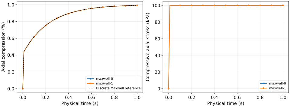
The axial stress stays near kPa. The axial strain continues beyond the first step, reaching about −0.00991968 at 1 s, or 9.920 mm equivalent shortening. Coordinates remain fixed; the script integrates the top velocity to reconstruct displacement.
Independent discrete reference
For homogeneous confined compression, let , be the signed mean normal stress, and the axial deviatoric stress, so . Start with . For the prescribed axial traction Pa, define
Crank–Nicolson integration of the Maxwell deviatoric response gives
These are algebraic homogeneous equations, independent of the mesh force assembly. The analysis script implements this recurrence and checks all elements, rather than using one PT option as the reference for the other.
This is a check against the discrete material update at the selected physical timestep. Agreement does not establish physical-time convergence. For the corresponding continuum step-load problem, the post-loading strain is
The instantaneous elastic jump is ; the long-time strain is . The first saved DES step includes a finite interval of creep, so it is not exactly that instantaneous jump. A timestep-refinement study against this continuum solution is a separate accuracy assessment. The provided plotting script expects the supplied 100-step, 0.01 s configs.
What this demonstrates
The held elastic and Maxwell runs test different physical responses. For elasticity, zero free velocity can preserve a completed loading increment. For Maxwell rheology, the same candidate still evaluates constitutive relaxation over the physical dt; a zero-velocity shortcut cannot suppress creep. Both PT schemes must recover the discrete history.
For the matching 3D exercise, use the 3D build and a fresh output directory as described in the elastic tutorial. The same inputs and analysis script apply.
These homogeneous, dry, fixed-grid checks do not qualify moving meshes, localized softening, arbitrary irreversible loading or hydraulic coupling. For solver controls and known convergence limits, return to Choosing a mechanical solver and the validation record.