Initial conditions from Geodynamic World Builder
The Geodynamic World Builder (GWB, Fraters et al. 2019) describes a model's starting state as a list of features, continental and oceanic plates, subducting slabs, faults, mantle layers and plumes, each with its own temperature and composition models, in one JSON file, the world. DES can take three of its initial fields from a world: the temperature, the material of every marker and the weak zone. The same world then describes the model for DES and for other codes that read GWB, such as ASPECT.
| Dimension | 2D and 3D |
| Build | make ndims=2 usegwb=1 (and ndims=3), with GWB installed |
| Inputs | examples/gwb-subduction.cfg, gwb-slab-3d.cfg, gwb-core-complex.cfg and their .wb worlds, added by DynEarthSol #117 |
| Checked with | revision not recorded on this page |
What you will learn
- How to build DES with GWB, and the three input options that use a world
- How DES queries the world, and what a world must contain to set materials
- How GWB faults become DES weak zones, and two conventions of GWB faults that matter for that
- Three examples: a 2D subduction zone, a 3D slab, and a 2D core complex whose weak zone alone comes from GWB
Prerequisites
- ✅ GWB (CMake 3.5 or newer, a C++14 compiler) built as a shared library and
installed, in under a minute on 4 cores:
The
git clone https://github.com/GeodynamicWorldBuilder/WorldBuilder.git
cmake -S WorldBuilder -B WorldBuilder/build -DCMAKE_BUILD_TYPE=Release \
  -DBUILD_SHARED_LIBS=ON -DWB_ENABLE_TESTS=OFF -DWB_ENABLE_PYTHON=OFF \
  -DWB_MAKE_FORTRAN_WRAPPER=OFF -DCMAKE_INSTALL_PREFIX=$HOME/opt/WorldBuilder
cmake --build WorldBuilder/build -j 4
cmake --install WorldBuilder/buildOFFoptions skip parts DES does not use; with Python on, the install also runs GWB'ssetup.py installinto the active Python. GWB installs its library inbin/, notlib/. Itsgwb-dat, which prints a world's fields at given points, is not installed and stays inWorldBuilder/build/bin/. - ✅ DynEarthSol with GeoFLAC/DynEarthSol#117,
which adds option 936, built with
usegwb=1(andGWB_DIRif GWB is not in~/opt/WorldBuilder); see Build:make ndims=2 usemmg=1 usegwb=1 GWB_DIR=$HOME/opt/WorldBuilder - ✅ For the figures: Python 3 with
numpyandmatplotlib
How it works
One input names the world, ic.gwb_filename. Option 936 of three [ic]
options takes a field from it; any of them can be used alone or together with
DES's other options. (936 reads as "gwb": 9 is a g, 3 on its side a w, 6 a b.)
| Option | Field | From the world |
|---|---|---|
temperature_option = 936 | temperature of every node | GWB temperature |
mattype_option = 936 | material of every marker | GWB composition i is mattype i |
weakzone_option = 936 | weakzone_plstrain in the weak elements, uniform or (with gwb_fault_is_gaussian) a Gaussian across the fault | the elements whose centroid lies in a GWB fault feature |
[ic]
gwb_filename = gwb-subduction.wb
temperature_option = 936
mattype_option = 936
weakzone_option = 936
weakzone_plstrain = 1
- Where the world is queried. A point of the initial mesh lies at depth −z,
since z = 0 is the surface. In 2D the world must have a
cross section, and DES's x is the distance along it; in 3D, DES's x and y are the world's map coordinates and no cross section is needed. - When. Only while the model is initialized; the world is then released.
A restart cannot re-seed its weak zone from the world:
is_restarting_weakzone = yeswithweakzone_option = 936is an error. - Remeshing. Materials ride on the markers, and temperature and plastic strain are carried over as usual. With MMG, DES refines the weak zone at t = 0, so a GWB fault also gets a finer initial mesh.
Writing a world for DES
Every point needs a material
GWB compositions are numbered 0, 1, 2, …; DES reads composition i as
mattype i, so number them in the order of the cfg's [mat] arrays. A marker
takes the composition that holds at least half of it. The world must give one
to every point of the domain, the mantle included: a marker with none, or with
only a composition ≥ num_materials, stops the run (exit 12) and names its
position and fractions.
In practice, give the mantle layer a composition of its own and fill each plate and slab below its crust:
{"model":"mantle layer", "name":"mantle", "max depth":300e3, "coordinates":[...],
 "composition models":[{"model":"uniform", "compositions":[2]}]},
{"model":"continental plate", "name":"overriding plate", "max depth":100e3, "coordinates":[...],
 "composition models":[{"model":"uniform", "compositions":[1], "max depth":35e3},
                       {"model":"uniform", "compositions":[2], "min depth":35e3, "max depth":100e3}]}
A later feature overrides an earlier one where they overlap, and a composition model replaces the compositions it does not list with zero.
Faults
Every fault feature is a weak zone. Two GWB conventions decide where:
- A fault starts at its
min depth. Itscoordinatesare the trace of the fault surface at that depth, not at the surface. A fault confined to 5–10 km depth on a plane that crosses the surface at x = 50 km and dips 60° has its trace at x = 50 − 5/tan 60° = 47.113 km. - Segment length plus thickness must reach the deepest point. A point
deeper than the fault's total segment length plus its thickness lies outside
it, even within
max depth. Make the segments long enough, and letmax depthend the fault.
A GWB fault's thickness is measured across the fault, while DES's
weakzone_halfwidth is measured horizontally: a planar DES zone of half-width
h dipping at θ is a GWB fault of thickness 2 h sin θ.
A fault without composition or temperature models changes neither, so a plate-interface fault can be added on top of the materials and temperatures above it.
By default every element in a fault gets the same weakzone_plstrain. With
ic.gwb_fault_is_gaussian = yes, the plastic strain falls off away from the
fault's plane as a Gaussian,
plstrain = weakzone_plstrain × exp(−d² / 2σ²)
where d is the element centroid's distance from the plane (GWB measures it
across the fault, like the thickness) and σ is ic.weakzone_standard_deviation,
in metres. The fault's thickness still bounds the zone, so make it about 4–6 σ
for the strain to fade before the edge. An element in several faults takes the
largest value; GWB finds each fault's plane by its name, so the faults need
distinct names.
Temperature
Set bc.mantle_temperature to the world's potential mantle temperature. DES
also takes the bottom temperature as the largest initial temperature.
Initial stress
DES starts from a lithostatic stress, the reference pressure of
control.ref_pressure_option, which the side walls and the Winkler bottom also
use. The examples take it from the mantle (ref_pressure_option = 0,
mat.mattype_ref = 2). PREM's (option 1) is interpolated between table rows
35 km apart whose rounding gives each interval a slightly different density;
the excess over the model's own weight then steps at every row, which shows as
horizontal stripes, at 80, 115, 150 and 185 km depth, in a quiet model's strain
rate.
Example 1: a 2D subduction zone
examples/gwb-subduction.cfg and .wb: a 600 × 200 km cross section of a
continental plate (35 km crust), an oceanic plate (7 km crust) and a slab
descending from x = 450 km to about 180 km depth, with GWB's plate and
mass-conserving slab temperatures, and a 12 km-thick fault along the slab top to
80 km, the plate interface. All three options are on; the materials are
0 oceanic crust, 1 continental crust and 2 mantle. The weak zone is Gaussian:
weakzone_plstrain = 1
gwb_fault_is_gaussian = yes
weakzone_standard_deviation = 2.5e3   # the 12 km thickness is about 5 sigma
cd DynEarthSol/examples
../dynearthsol2d gwb-subduction.cfg
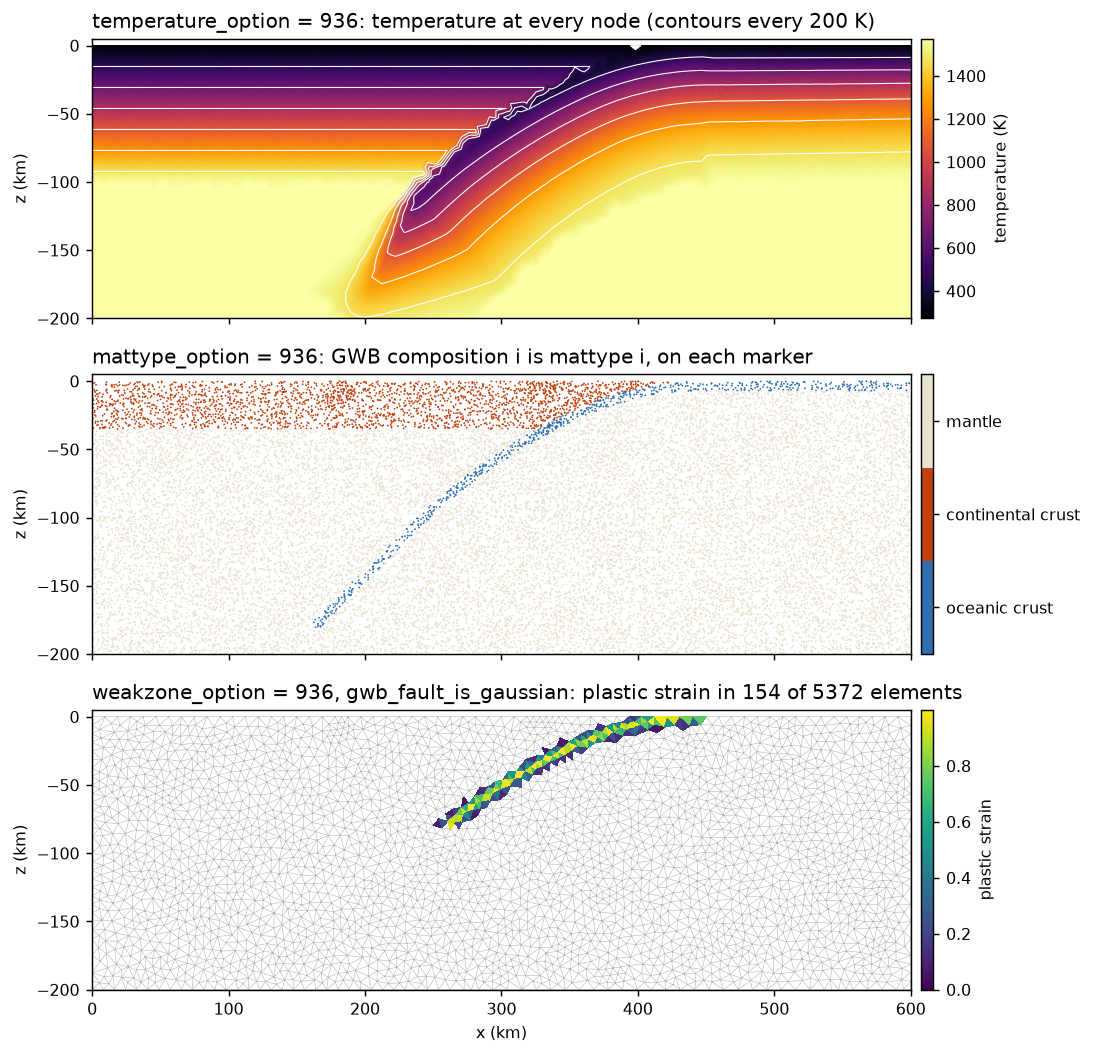
The initial mesh has 5372 elements and 21 488 markers: 743 of oceanic crust, 2443 of continental crust and 18 302 of mantle. 154 elements lie in the fault, with plastic strain from 1 at the slab top down to 0.06 at the fault's edges, 6 km away. The ragged isotherms above the slab follow a step in the world's temperature at the slab top: at x = 330 km it drops by 285 K within 1 km at 33 km depth, from the overriding plate's geotherm to the cold slab, and the 5 km mesh samples that step. The example runs 100 kyr with fixed walls in about 8 s on 4 threads: it shows the initial fields rather than subduction.
Example 2: a weak zone alone, in a core complex
examples/gwb-core-complex.cfg is the bundled core-complex.cfg, the model of
Tectonic rifting and subduction Part 1, with only its seed
fault taken from a world. Temperature and the single material stay DES's own:
[ic]
weakzone_option = 936
weakzone_plstrain = 0.5
gwb_filename = gwb-core-complex.wb
{"model":"fault", "name":"seed fault", "min depth":5e3, "max depth":10e3,
 "coordinates":[[47.113e3,-100e3],[47.113e3,100e3]], "dip point":[0,0],
 "segments":[{"length":12e3, "thickness":[2.08e3], "angle":[60]}]}
The fault reproduces the planar weak zone of core-complex.cfg: the plane
through (50 km, 0) dipping 60° toward −x, between 5 and 10 km deep, with the
1.2 km horizontal half-width as a 2 × 1.2 × sin 60° = 2.08 km thickness. Both
fault conventions above are at work: the trace is where the plane reaches the
5 km min depth, and the 12 km segment is longer than the 10 − 2.08 km it
must reach.
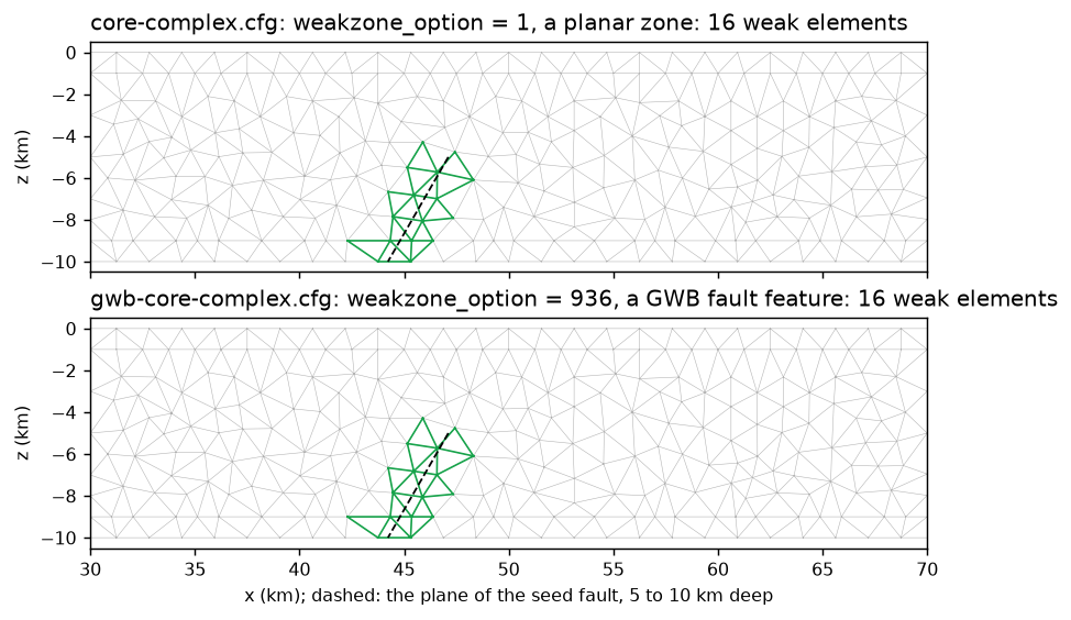
The two runs start from the same mesh, refined by MMG around the same 16 weak elements, and stay identical: frame 3 matches bit for bit.
Example 3: a 3D slab
examples/gwb-slab-3d.cfg and .wb: a 200 × 100 × 100 km box with a
continental plate (30 km crust) for x < 80 km, an oceanic plate (7 km crust)
beyond, a slab dipping from the trench at x = 80 km, and a 10 km-thick fault
along its top to 60 km depth. In 3D the world has no cross section.
../dynearthsol3d gwb-slab-3d.cfg
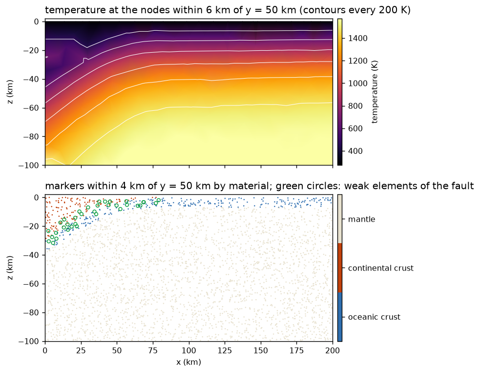
The mesh has 10 131 elements and 40 524 markers (3089 oceanic crust, 1807 continental crust, 35 628 mantle); 427 elements lie in the fault. The front and back faces are free slip: left free, they bulge outward, since the plates and the slab weigh differently and no one reference pressure holds them all. The example runs 5 kyr in about 6 s on 4 threads. Run it longer and the dense slab sinks along the weak interface at velocities far above the 3.15 cm/yr push, and the mesh is remeshed often.
Errors
| Symptom | Cause |
|---|---|
exit 31: ... 936 needs the Geodynamic World Builder: build with usegwb=1 | DES was built without GWB |
exit 11: ... 936 needs ic.gwb_filename | no world named |
exit 20: cannot open ic.gwb_filename | the world file is missing |
exit 11: ic.weakzone_option 936 cannot re-seed the weak zone of a restart | a restart with is_restarting_weakzone = yes |
exit 11: Error: Geodynamic World Builder, world '...': ... | GWB rejected the world; its own message follows. In 2D, a world without a cross section is one cause |
exit 12: ... defines no material at x = (...) | mattype_option = 936 and a marker without a composition of at least 0.5 below num_materials; see Every point needs a material |
exit 12: ic.weakzone_option 936 needs a fault feature | the world has no fault |
exit 12: ic.gwb_fault_is_gaussian needs the faults ... to have distinct names | two faults share a name |
exit 11: ic.gwb_fault_is_gaussian needs ic.weakzone_standard_deviation > 0 | σ is 0 or negative |
Testing
DynEarthSol's GWB build workflow builds GWB at a pinned commit, builds DES
in 2D and 3D with usegwb=1, and runs tests/functional/gwb/check_gwb.py. The
script compares frame 0 of a 2D and a 3D world with GWB's own gwb-dat
application point by point: every node temperature, every marker's material
and every weak element. It also checks the error exits above.
References
- Fraters, M., Thieulot, C., van den Berg, A. & Spakman, W. (2019). The Geodynamic World Builder: a solution for complex initial conditions in numerical modeling. Solid Earth, 10, 1785–1807. doi:10.5194/se-10-1785-2019