Tectonic rifting and subduction
This tutorial walks through two classic long-term tectonic models with DynEarthSol: rifting of a brittle crustal layer, which produces a metamorphic core complex, and subduction of an oceanic plate beneath an overriding plate. Both use bundled 2D examples as a starting point, so you can run them as they are and then modify one ingredient at a time.
Both cases move material a long way under divergent or convergent forcing. Deformation localizes where plastic strain accumulates, and with MMG remeshing the mesh is refined there, so faults stay sharp as the model runs. The first case takes minutes on a laptop; the second about half an hour.
| Dimension | 2D |
| Build | make ndims=2 usemmg=1 |
| Run time | 12 minutes (rifting, to 100 kyr) and 22 minutes (subduction, to 5 Myr) on 6 threads |
| Inputs | examples/tectonics/core-complex.cfg, examples/tectonics/subduction.cfg and the tutorial package |
| Checked with | Part 1: DynEarthSol 68cc2a0 (relief, dip and element count as stated); Part 2: DynEarthSol 68cc2a0 (slab-tip depths, mesh growth and step count as stated; serpentinite and eclogite counts within 10 %; deepest trench point about 1 km deeper than stated, within the run-to-run scatter described under Exercise 3) |
What you will learn
- How a DES
.cfgfile is organized and which sections matter for tectonics - How Mohr–Coulomb plasticity with strain softening produces faults, and how a weak zone and the wall velocities decide where and how fast
- How a slab-shaped initial geometry is built with a
.polyfile - How marker phase changes add serpentinite and eclogite as the slab descends, and what the virtual-topology grid does for them
- How remeshing keeps a Lagrangian mesh usable, what triggers it, and how MMG refines along the faults and the plate interface
- How to read the output: plastic strain, topography, viscosity, temperature, material and velocity
- How to restart a run from a checkpoint with a changed boundary condition, and read what the model does when its forcing stops
The two parts are meant to be read in order. Part 1 is the smallest model that shows a DES fault: one material, no temperature, a box mesh, a planar seed, three run steps. Part 2 keeps that skeleton and adds one ingredient at a time:
| Ingredient | Part 1: core complex | Part 2: subduction |
|---|---|---|
| Geometry | A box, refined in the middle by the config | A .poly file with a slab already in the mantle |
| Materials | One | Six populated, four reserved for phase-change products |
| Rheology | Elasto-plastic | Elasto-visco-plastic with a geotherm |
| Seed | One planar weak zone | One dipping segment along the slab top |
| Walls | Both pulled apart | One pushed in, one fixed; material flows in through the wall |
| Phase changes | None | Serpentinization and eclogitization on a marker grid |
| Remeshing | Bottom restored | Bottom and side walls restored, which needs MMG |
| Run time, 6 threads | 12 minutes to 100 kyr | 22 minutes to 5 Myr |
Every run time quoted on this page is the wall-clock time on 6 threads of an Apple M3 Max laptop; a 4-core machine of a few years ago takes two to three times longer.
Each part has the same four steps, geometry, configuration, run, and what to look for, followed by exercises that change one parameter at a time.
For a hands-on class, download the tutorial package (12 MB).
It holds a Jupyter notebook that draws every figure of this page, the configs
of both parts and all exercises with the shell commands to run them, and
reference results so the plots work before your own runs finish. Start with its
README; resources/SETUP.md has a short build recipe.
Prerequisites
This tutorial follows the ones before it in this section and uses what they cover. Before starting, ensure you have:
- ✅ DynEarthSol compiled in 2D with MMG,
make ndims=2 usemmg=1; see Build and Running DES3D. MMG is a git submodule thatmakefetches and builds for you; the build is described in Adaptive mesh refinement with MMG - ✅ Python 3 with
numpyfor2vtk.py, and ParaView or another VTK viewer; see Visualizing outputs - ✅ Read Making a complex mesh with
.polyfile: Part 2 reads its slab geometry from one - ✅ Read Weak zones: Part 1 seeds a fault with a planar weak zone and Part 2 the plate interface with a segment one
Velocity boundary conditions (3D) and Rate-and-state friction are not needed here: both examples are 2D with steady wall velocities and no earthquake cycles. The next tutorial, Coupling with GoSPL, adds surface processes to models like these.
A plain make builds the 3D executable without MMG, and that is what the
build instructions and the first tutorial leave you with. This tutorial needs
the 2D MMG build, make ndims=2 usemmg=1, which takes a few minutes on a
laptop and leaves the 3D executable in place. Check it with
./dynearthsol2d --help | grep -c mmg, which must print a number above zero.
Part 2 also needs a source tree from after 30 October 2026; see its note.
Both examples are 2D; a 3D build (make) runs the same physics at a much
higher cost. Part 1 runs on either build: a plain Triangle build
(make ndims=2) remeshes uniformly, an MMG build refines along the fault,
and the MMG box in Part 1 says what changes. Part 2 needs the MMG build,
because its restored side walls (remeshing_option = 13) are only available
with MMG. If you build once, build with usemmg=1.
How the model works
DynEarthSol's rheology is built from three responses that can be switched on
per run with rheology_type. Part 1 uses elasto-plastic; Part 2 adds
viscous creep with elasto-visco-plastic.
| Component | Controls | Key parameters | Used in |
|---|---|---|---|
| Elastic | Short-term stress build-up | bulk_modulus, shear_modulus | Parts 1 and 2 |
| Plastic (Mohr–Coulomb, strain softening) | Brittle faulting | cohesion0/1, friction_angle0/1, dilation_angle0/1, pls0/1 | Parts 1 and 2 |
| Viscous (power-law creep) | Ductile flow where it is hot | visc_exponent, visc_coefficient, visc_activation_energy, min_viscosity, max_viscosity | Part 2 only |
| Temperature | Viscosity through creep; density through alpha | temperature_option, oceanic_plate_age_in_yr, surface_temperature, mantle_temperature | Part 2 only |
| Phase changes | Marker material conversion at pressure–temperature boundaries | phase_change_option, mattype_*, has_serpentinization, has_eclogitization | Part 2 only |
Strain softening
Faults in DES are bands of elements that have yielded. A band localizes only
if the material gets weaker as it deforms: cohesion and friction angle drop
linearly from their 0 values to their 1 values as accumulated plastic
strain goes from pls0 to pls1. Fast softening (small pls1) favours one
long-lived fault; slow softening spreads deformation over many short-lived
faults.

Seeding deformation: the weak zone
In a uniform model nothing selects where the first fault forms, so the
location of localization is uncontrolled and depends on mesh noise. A weak
zone is a region given an initial plastic strain weakzone_plstrain, which
pre-softens it and pins the first fault. Part 1 uses a planar seed
(weakzone_option = 1), Part 2 a dipping multi-segment one. The other shapes
are described in Weak zones.
Driving deformation: velocity boundary conditions
vbc_x0 and vbc_x1 set the condition type on the left and right walls; type
1 fixes the normal velocity and leaves the shear component free. vbc_val_x0
and vbc_val_x1 are the normal velocities in m/s, positive toward +x, so a
negative value on the left wall and a positive one on the right wall pull the
model apart. The top is a free surface. The bottom carries a Winkler
foundation, a lithostatic normal stress that lets the base move vertically.
Thermal structure (Part 2)
Part 1 is isothermal. Part 2 sets an initial geotherm by half-space cooling
(temperature_option = 0, oceanic_plate_age_in_yr), and temperature then
evolves by conduction and advection. It feeds back into the viscosity through
the creep law, which is what makes the deep slab and the mantle wedge flow.
The other options are for continents: 1 is a linear continental gradient
over lithospheric_thickness, 2 adds the equilibrium of crustal radiogenic
heating, 3 puts an adiabatic mantle under the continental gradient, and 90
reads a temperature grid from a file.
Remeshing and markers
A Lagrangian mesh follows the material, so elements distort as faults slip.
When the worst element quality drops below min_quality (checked every
quality_check_step_interval steps), or a boundary moves by more than
max_boundary_distortion × resolution, DES rebuilds the mesh and maps the
fields onto it. remeshing_option = 11 restores the bottom boundary to its
initial depth. Markers carry material identity across remeshes. With MMG the
rebuild is adaptive: elements are sized from accumulated plastic strain, so
faults get finer elements and the quiet far field stays coarse. See
Remeshing and MMG.
Part 1: Rifting a brittle crust (core complex)
The bundled example
examples/tectonics/core-complex.cfg
stretches a single 10 km brittle layer with a pre-cut dipping fault. With
strain softening the fault keeps slipping, its footwall rises and rotates,
and the fault surface flattens into a dome. This is the rolling-hinge
mechanism of metamorphic core complexes (Lavier, Buck & Poliakov 1999), and
it is the fastest way to see every ingredient of a DES tectonic run.

| Setting | |
|---|---|
| Domain | 100 × 10 km, 1 km resolution refined in the central 40 km (meshing_option = 2, refined_zonex = [0.3, 0.7]) |
| Forcing | ±1e-9 m/s (3.15 cm/yr per side, 6.3 cm/yr total) extension in x |
| Duration | 50 kyr as shipped (3.2 km of total extension), output every 1.5 kyr |
| Rheology | elasto-plastic, one material (ρ = 2700 kg/m³), cohesion 44 → 4 MPa over 0.5 plastic strain, friction 30° fixed |
| Weak zone | Planar (weakzone_option = 1), dipping 60°, 1.2 km half-width, in the lower half of the layer at x = 50 km |
| Surface | Hillslope diffusion, surface_diffusivity = 1e-7 m²/s |
| Thermal | Isothermal, 273 K |
Step 1: The initial geometry and mesh
Part 1 needs no mesh file. The box, its refinement and the seed fault are all
set in the config: meshing_option = 2 meshes a rectangle at resolution
between refined_zonex = [0.3, 0.7], 30 to 70 km, and lets elements grow to
largest_size times the area outside, about 3 km on an edge. The seed is a
planar weak zone through (50 km, 0) dipping 60° toward −x, 1.2 km wide and
confined to the lower half of the layer, where it is given a plastic strain
equal to pls1 so it starts fully softened.

Step 2: The configuration
[sim]
modelname = result3
max_time_in_yr = 50000
output_time_interval_in_yr = 1500
has_output_during_remeshing = no
is_outputting_averaged_fields = no

[mesh]
meshing_option = 2
xlength = 100e3
ylength = 10e3
zlength = 10e3
resolution = 1e3
largest_size = 10
smallest_size = 0.01
refined_zonex = [0.3, 0.7]
refined_zoney = [0.0, 1.0]
refined_zonez = [0.0, 1.0]
quality_check_step_interval = 500
remeshing_option = 11

[control]
surface_process_option = 1
surface_diffusivity = 1e-7
dt_fraction = 1.0
inertial_scaling = 1e5

[bc]
vbc_x0 = 1
vbc_x1 = 1
vbc_val_x0 = -1e-9
vbc_val_x1 = 1e-9
vbc_y0 = 1
vbc_y1 = 1
vbc_val_y0 = 0
vbc_val_y1 = 0
has_water_loading = no
surface_temperature = 273
mantle_temperature = 273

[ic]
weakzone_option = 1
weakzone_azimuth = 15
weakzone_inclination = -60
weakzone_halfwidth = 1.2
weakzone_depth_min = 0.5
weakzone_depth_max = 1.0
weakzone_xcenter = 0.5
weakzone_ycenter = 0.5
weakzone_zcenter = 0
weakzone_plstrain = 0.5

[mat]
rheology_type = elasto-plastic
rho0 = [2700]
alpha = [0]
bulk_modulus = [50e9]
shear_modulus = [30e9]
pls0 = [0]
pls1 = [0.5]
cohesion0 = [4.4e7]
cohesion1 = [4e6]
friction_angle0 = [30]
friction_angle1 = [30]
min_viscosity = 1e24
Section by section:
[sim]names the output (result3.save.*) and runs 50 kyr with a frame every 1.5 kyr. Instantaneous rather than averaged fields are written.[mesh]builds a 100 × 10 km box.meshing_option = 2refines the central 40 % in x atresolution, and lets the flanks coarsen up tolargest_sizetimes that.ylengthis read but unused in 2D.remeshing_option = 11flattens the bottom back to 10 km depth at every remesh.[control]turns on surface diffusion and sets the mass scaling.inertial_scalingis the factor by which density is inflated to lengthen the elastic time step; see Mass scaling. With no viscosity in play, this parameter and the element size setdt.[bc]pulls the two walls apart at 3.15 cm/yr each. Thevbc_y*lines matter only in 3D. Water loading is off because the surface starts at sea level and would otherwise be loaded as it subsides.[ic]cuts the seed fault. Positions are fractions of the domain:weakzone_xcenter = 0.5is x = 50 km, andweakzone_depth_min/max = 0.5, 1.0confines the seed to the lower 5 km.weakzone_halfwidthis in units ofresolution.weakzone_plstrain = 0.5equalspls1, so the seed starts fully softened.weakzone_azimuthis a 3D parameter and is ignored here.[mat]is one material. Cohesion softens by a factor of 11; friction does not.min_viscosityis irrelevant forelasto-plasticbut must be set.
The parameters you will change most often:
| Parameter | What it sets |
|---|---|
max_time_in_yr | Total extension; 100 kyr gives 6.3 km and a clear dome |
weakzone_inclination | Dip of the seed fault; the sign picks which way it dips |
pls1 | Plastic strain needed to fully soften; smaller localizes faster |
cohesion1 | Strength after softening; lower = sharper fault |
surface_diffusivity | How fast relief is smoothed; controls footwall exhumation |
vbc_val_x0, vbc_val_x1 | Extension rate at each wall, m/s |
resolution, refined_zonex | Element size and where it is fine |
Step 3: Run
cd DynEarthSol/examples/tectonics
OMP_NUM_THREADS=6 ../../dynearthsol2d core-complex.cfg
As shipped the file stops at 50 kyr, which is enough to see the fault break through and the footwall start to rise. The figures below run to 100 kyr, when the dome is fully formed; to reproduce them, change one line:
max_time_in_yr = 100000
The log prints one line per output_time_interval_in_yr with the step count,
model time and dt, and a remeshing notice whenever the mesh is rebuilt.
Output goes to result3.save.* and result3.info in the working directory.
Cost on a laptop: the stock 50 kyr run takes a few minutes. To 100 kyr the
MMG build took 12 minutes on 6 threads while another run shared the machine,
6.2 million steps, 23 remeshes, 720 to about 1300 elements. The Triangle build
needs about the same number of steps and ends with about 1800 elements. It
remeshes some 20 times for the usual reasons, but twice in the run a surface
element at the fault scarp, x = 53 km, sits just below min_quality after
each rebuild, so every quality
check remeshes again, over 1100 times in all. Remeshing is still about 1 % of
the wall time with Triangle and 0.03 % with MMG; the time step, not the mesh,
is the cost.
The runs shown below use the MMG build from the prerequisites. The same file
also runs on a plain Triangle build (make ndims=2); nothing in the config
changes. The difference is in how the mesh is rebuilt. MMG sizes elements
from accumulated plastic strain, within a band set by two parameters the file
already has: the largest edge is resolution × largest_size^(1/2) and the
smallest resolution × (smallest_size × mmg_remesh_defensive_tiny_ratio)^(1/2),
3.2 km and 0.12 km here, and it is conservative, freezing elements that are
not yielding, distorted or tiny so that each remesh touches mainly the fault
band. Triangle rebuilds the whole mesh at the initial sizes. To 100 kyr the
MMG run ends with about 1300 elements after 23 remeshes, the Triangle run
with about 1800 after over 1100, nearly all of them repeats on a surface
element at the fault scarp that a rebuild does not improve.
The build is described in Adaptive mesh refinement with MMG.
The full parameter list, with a one-line tuning rule for each, is in the
[mesh] section of
examples/defaults.cfg
and in dynearthsol2d --help. These parameters are in DynEarthSol master
since PR #95, October 2026.
Step 4: What to look for
python ../2vtk.py result3
Open result3.*.vtu in ParaView. Fields to look at:
- plastic strain, the fault, and whether it stays one band
- surface topography, footwall uplift and hanging-wall basin
- strain rate, where slip is happening now, as opposed to where it has happened
- the mesh itself, how element size tracks the fault after remeshing
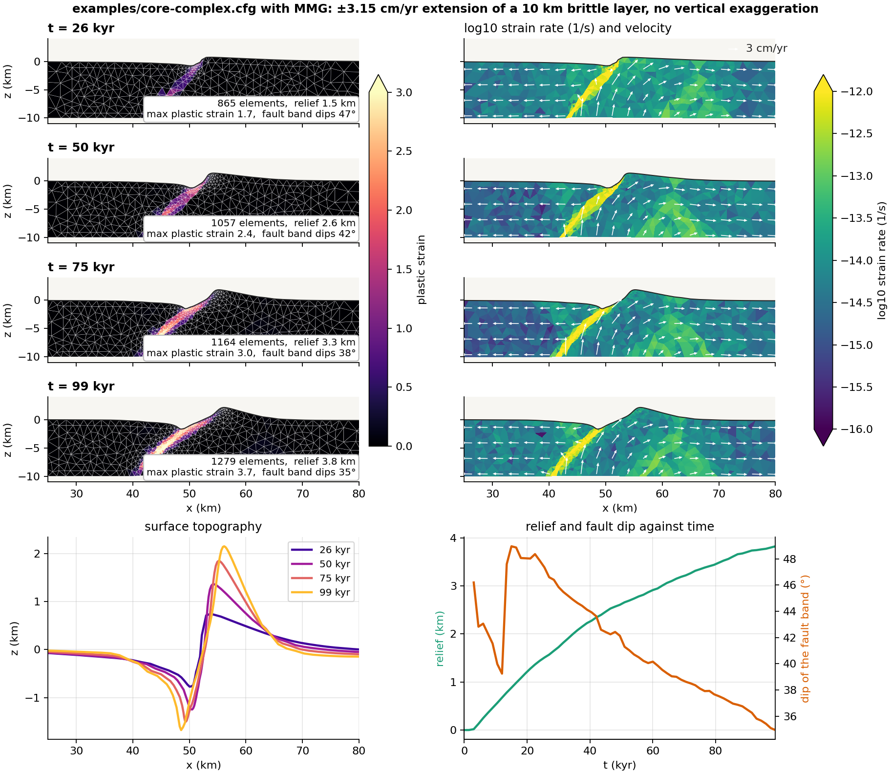
The left column is where slip has accumulated and how the mesh follows it; the right column is where slip is happening now. They differ: at 50 kyr the strain rate shows a second, antithetic band under the footwall at x = 55–65 km that never gains enough plastic strain to show on the left. The bottom row quantifies the rolling hinge: the fault band steepens to 49° while it breaks through, then rotates steadily to 35° by 100 kyr as relief grows to 3.8 km.
Things to look for as the run proceeds (the figure is the reference run):
- Breakthrough. The seed fault cuts up to the surface at about 13 kyr and the footwall starts to rise; the velocity arrows show the footwall moving up and to the right while the hanging wall slides left.
- Relief. By 50 kyr the surface has a footwall crest of 1.4 km near x = 54 km and a basin of 1.2 km near x = 50 km, 2.6 km of relief; by 100 kyr the crest is 2.2 km at x = 56 km and the relief 3.8 km.
- The rolling hinge. The fault rotates to a shallower dip as it is exhumed, from about 47° at 25 kyr to 35° at 100 kyr; the band of high plastic strain curves from steep at depth to gentle near the surface, and its exhumed upper part drapes the footwall dome.
- The mesh. After a remesh the elements along the fault are smaller than in the far field with MMG, and uniform with Triangle; the MMG run grows from 720 to about 1300 elements over 100 kyr.
Exercise 1: change the surface diffusivity
| Run | surface_diffusivity | What you should see at 100 kyr |
|---|---|---|
| Reference | 1e-7 | Sharp footwall crest 2.2 km high, basin 1.7 km deep, 3.8 km of relief |
| Moderate | 1e-6 | The same structure a little smoothed: crest 1.8 km, basin 1.6 km, 3.4 km of relief |
| Strong erosion | 1e-5 | Relief capped at 1.5 km from about 50 kyr on; the crest is planed to 1 km and the basin filled to 0.5 km while the fault keeps slipping |
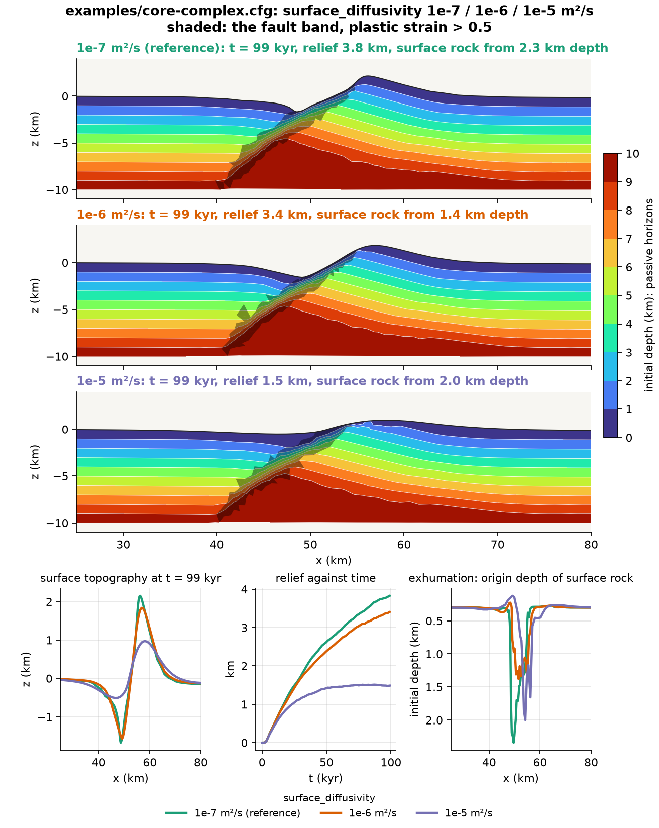
The coloured bands are passive horizons: every node carries its initial
position through remeshing in the coord0 field, so contouring the initial
depth on the present mesh shows where each layer of the original crust has
gone. Read them together with the surface panels:
- The fault is the same in all three runs. The band dips 41° to 42° at 50 kyr and 34° to 36° at 100 kyr and reaches a plastic strain of 3.7 whatever the diffusivity. Diffusion acts on the surface only.
- So is the exhumation. Rock from 8 km depth has risen to about 4 km depth at x = 48 km in all three, the horizons under the dome are bent the same way, and the rock exposed at the surface came from 1.4 to 2.3 km in every run. The fault sets how far the footwall rises; erosion does not add to it here.
- What changes is the topography. At 1e-5 m²/s the relief stops growing at about 50 kyr because the crest is planed as fast as the fault lifts it and the debris fills the basin. The same exhumation then shows as a low dome rather than a sharp crest.
That is why relief alone is a poor measure of what a fault has done, and why the horizons are worth drawing. Each run took 4 to 12 minutes on 6 threads.
Exercise 2: change how small the elements may get
Requires the MMG build (make ndims=2 usemmg=1). Two parameters decide how
fine the mesh becomes along the fault. smallest_size is the area of the
smallest allowed element relative to one of edge resolution: with MMG it
sets the floor of the refinement band,
resolution × (smallest_size × mmg_remesh_defensive_tiny_ratio)^(1/2), and
for every remesher it sets the tiny-element trigger, an element compressed
below smallest_size of its nominal area forcing a remesh. Both scale with
its square root, so a factor of 100 in smallest_size is a factor of 10 in
element edge. mmg_metric_refine_coeff is the target: MMG aims for an
element area of the initial one divided by 1 + coeff × plastic strain, so
at the default 5 an element at a plastic strain of 4 is asked to shrink to a
fifth of its initial edge. The mesh can only be as fine as the target asks
and the floor allows.
| Run | smallest_size | Smallest MMG element | What you should see |
|---|---|---|---|
| No refinement | 1 | 1.2 km | A diffuse band 3 km wide that never sharpens; the run takes an eighth of the time |
| Stock | 0.01 | 0.12 km | A sharp fault, about 1300 elements; 12 min |
| Very fine | 0.001 | 0.04 km | The same mesh as stock, since the target rather than the floor limits refinement; 5 % more steps for nothing |
| Very fine, stronger target | 0.001 with mmg_metric_refine_coeff = 10 | 0.04 km | Now the band refines: 1770 elements, 70 % more in the band, and a second fault splays into the hanging wall |
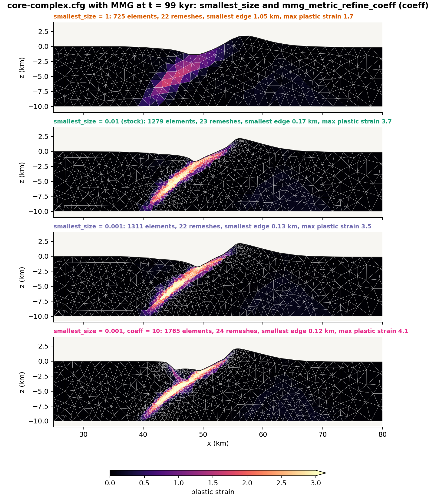
All four rows were run. Going up to smallest_size = 1 costs resolution:
the fault still forms in the same place and the surface still domes, but
the band cannot be narrower than the elements it runs through, so the strain
is spread over a 3 km wide zone and the fault never sharpens. The time step
is on average seven times longer, since it follows the smallest element, and
the whole run takes an eighth of the time.
Going down to 0.001 alone buys nothing. The smallest element in the stock
run is 0.17 km, above the 0.12 km floor, so the floor was not what stopped
the refinement; the target was. Lowering the floor further cannot refine the
band, and what it does change is the tiny-element trigger: squeezed elements
may now shrink to a third of the size before a remesh repairs them, so the
time step can fall further. Here that costs only 5 % more steps, but it is a
cost with nothing in return.
Raising the target as well, mmg_metric_refine_coeff = 10, is what makes
the lower floor useful. The band now holds 560 elements instead of the stock
run's 330, at a median edge of 0.29 km instead of 0.43, and the smallest element reaches
0.12 km, still above the 0.04 km floor. The fault is drawn more sharply and
the maximum plastic strain is a little higher, 4.1 against 3.7. The finer
band also lets a second fault split off the main one into the hanging wall
from about 50 kyr; by 100 kyr it reaches the surface at x = 45 km and opens
a second, smaller basin there.
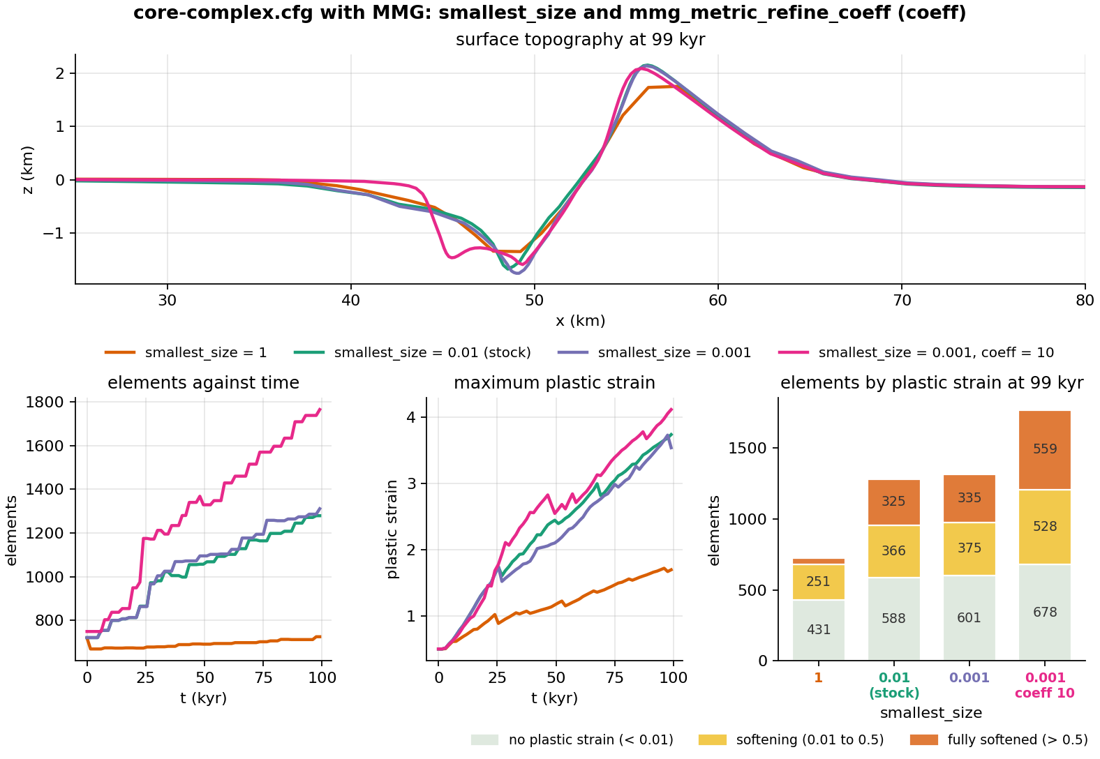
Away from that splay the surface hardly notices: the three refined runs end with the same crest and basin to within 0.2 km, and only the unrefined run is lower and broader. The lesson is that the two parameters work as a pair: the target asks for refinement where plastic strain accumulates, the floor caps how far it may go, and moving one without the other changes the cost of the run more than its result.
Change one parameter at a time, and keep a log of what you changed.
Going further: a lithospheric rift
core-complex.cfg has no mantle, no temperature and no viscosity.
examples/tectonics/rifting-2d.cfg
adds all three: a 500 × 150 km crust-over-mantle lithosphere read from a
.poly file (the one used in Making a complex mesh),
elasto-visco-plastic rheology, a 100 Myr half-space geotherm and a Gaussian
weak zone. It runs for 2 Myr at 6 km resolution. Everything in Part 2 that
is new relative to Part 1 appears there first, so it is a good intermediate
step.
Part 2: Subduction
The example below, examples/tectonics/subduction.cfg, and the phase-change engine it
uses (phase_change_option = 3 on a virtual-topology marker grid) reached
DynEarthSol master on 30 October 2026 with
pull request #110. A clone
or build from before that date does not have them: git pull and rebuild
with make ndims=2 usemmg=1 first. A quick check is
./dynearthsol2d --help | grep -c serpentinization, which must print a
number above zero.
The example
examples/tectonics/subduction.cfg
with its mesh file poly-subduction.poly pushes an oceanic plate under a
fixed overriding plate. A short slab is already in the mantle at the start,
so the plate interface exists from the first step. Two metamorphic reactions
run on the markers as the slab descends: mantle just above the slab top
becomes serpentinite, a weak and light layer that lubricates the
interface, and slab crust that sinks past the basalt-to-eclogite boundary
becomes eclogite, dense enough to add slab pull. Everything that was
missing from Part 1 appears here: several materials, viscous creep, a
geotherm, a .poly geometry, phase changes and material flowing in through
a side wall.
| Setting | |
|---|---|
| Domain | 400 × 160 km, 6 km resolution, a 10 km halo of refined mantle around the slab (poly-subduction.poly) |
| Initial slab | Oceanic crust 7 km thick, from the trench at x = 125–139 km dipping 30° to 40 km depth |
| Forcing | Left plate pushed at +1e-9 m/s (3.15 cm/yr) into a fixed right wall (vbc_val_x1 = 0) |
| Duration | 5 Myr, a frame every 50 kyr; about 23 min alone on 6 threads, 31 min when two runs share the machine; 5.8 million steps |
| Rheology | elasto-visco-plastic, 10 materials of which 6 are populated; cohesion 40 → 4 MPa and friction 30° → 15° over 0.1 plastic strain; sediment and serpentinite at 3° |
| Phase changes | phase_change_option = 3: serpentinization and eclogitization on, the other rules off |
| Weak zone | One 30° segment along the slab top (weakzone_option = 5), seeding the plate interface |
| Thermal | Half-space cooling, 80 Myr plate; surface 273 K, mantle 1573 K |
| Remeshing | MMG required; remeshing_option = 13 restores the side walls so the incoming plate keeps its layering |
| Surface | Hillslope diffusion, surface_diffusivity = 5e-7 m²/s; deposits become sediment |
Step 1: The initial geometry and mesh
A subducting slab needs a pre-existing dipping interface, which a weak zone
alone cannot supply. poly-subduction.poly defines it as a region of oceanic
crust already inside the mantle, following
Making a complex mesh with .poly file:
 0------------------------------------------7  z = 0: top, free surface
 1------------------------------------------6  z = -2 km: sediment / crust
 2----12--8=====9--13-----------------------5  z = -9 km: crust / mantle
 |      \  \  0  \   \                      |
 |       \  10----11   15                   |  10-11: slab end, cut normal to the dip
 |        \         \ /                     |  12-14: halo below the slab
 |         14-------/                       |  13-15: halo above the slab
 |                                          |
 3------------------------------------------4  z = -160 km: bottom
| Region | Material | Max element area | What it is |
|---|---|---|---|
| 0 | 3, sediment | 4 km² | The top 2 km across the whole domain |
| 1 | 0, oceanic crust | 8 km² | 2 to 9 km depth across the whole domain |
| 2 | 0, oceanic crust | 8 km² | The slab, 7 km thick, 30° dip, ending at 34–40 km depth |
| 3 | 2, mantle | 10 km² | A 10 km halo around the slab, refined so the serpentinite layer is resolved |
| 4 | 2, mantle | 1000 km² | The rest of the mantle, coarse |
Three things to notice:
- No region holds serpentinite or eclogite. Those materials exist only because the phase-change rules create them.
- The halo is what makes the example affordable: 6 km elements everywhere except a band where the interface needs them finer.
- The internal segments are discarded at the first remesh
(
is_discarding_internal_segments = yes). After that the slab is carried by the markers alone, which is whyhas_marker_output = yesis set.
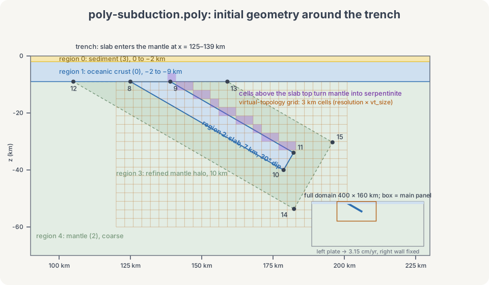
The grid drawn over the slab is the virtual topology used by the serpentinization rule, explained below. Its cells are half an element wide, so the one-element-thick slab crust gets its own row of crust-dominant cells instead of being averaged with the mantle.
Step 2: The configuration
[sim]
modelname = model-subduction
max_time_in_yr = 5e6
output_time_interval_in_yr = 50e3
has_marker_output = yes

[mesh]
meshing_option = 90
poly_filename = poly-subduction.poly
xlength = 400e3
zlength = 160e3
resolution = 6e3            # times vt_size = serpentinization grid cell
smallest_size = 0.04
quality_check_step_interval = 1000
min_quality = 0.2
remeshing_option = 13       # restore the side walls (needs MMG)
is_discarding_internal_segments = yes
mmg_hausd_factor = 0.1
max_boundary_distortion = 1
mmg_aniso_wall_ratio = 2

[markers]
init_marker_option = 1
replenishment_option = 12

[control]
ref_pressure_option = 1     # PREM
surface_process_option = 1
surface_diffusivity = 5e-7
inertial_scaling = 1e4

[bc]
surface_temperature = 273
mantle_temperature = 1573
vbc_x0 = 1
vbc_x1 = 1
vbc_val_x0 = 1e-9           # +x, 3.15 cm/yr
vbc_val_x1 = 0              # fixed backstop
has_water_loading = no

[ic]
weakzone_option = 5
weakzone_plstrain = 1
weakzone_num_segments = 1
weakzone_segments_inclination = [30]
weakzone_segments_halfwidth   = [0.6]
weakzone_segments_xcenter     = [0.42]
weakzone_segments_zcenter     = [0.135625]
weakzone_segments_depth_min   = [0.000]
weakzone_segments_depth_max   = [0.19375]
weakzone_segments_x_min       = [0.275]
weakzone_segments_x_max       = [0.575]
oceanic_plate_age_in_yr = 80e6

[mat]
rheology_type = elasto-visco-plastic
num_materials = 10
phase_change_option = 3
mattype_oceanic_crust = 0
mattype_mantle = 2
mattype_sediment = 3
mattype_serpentinite = 4
mattype_eclogite = 5
serpentinization_thickness = 5e3
#                 [ ocean0   (1)      mant2   sed3    serp4   eclg5  ... ]
rho0            = [ 2880,    2800,    3300,   2400,   3200,   3480,  ... ]
friction_angle0 = [ 30,      30,      30,     3,      3,      30,    ... ]
friction_angle1 = [ 15,      15,      15,     3,      3,      15,    ... ]
pls1            = [ 0.1 ]
max_viscosity = 1e24
min_viscosity = 1e19
Section by section, with what is new relative to Part 1:
[sim]writes a frame every 50 kyr and the markers with it, since the materials live on the markers once the poly segments are gone.[mesh]reads the.polyfile (meshing_option = 90).remeshing_option = 13restores the left and right walls to their initial positions at every remesh, so the plate entering through the left wall arrives with its sediment-over-crust-over-mantle layering intact. This option needs MMG.mmg_aniso_wall_ratio = 2lets the incoming column be carried on elements twice as long normal to the wall as along it.[markers]replenishment_option = 12refills an element that has lost its markers with its own single material, which keeps thin layers from vanishing.[control]ref_pressure_option = 1uses the PREM reference pressure; the phase-change rules read pressure and temperature at the marker's depth below the current free surface.inertial_scaling = 1e4lengthens the time step ten times over the default, buying speed at a known cost in accuracy, which the file's comments quantify.[bc]pushes only the left wall. The right wall is a fixed backstop, so the trench sits still in the model frame and the slab is fed from the left. The two temperatures set the half-space geotherm with the 80 Myr age in[ic].[ic]seeds the interface with a single 30° plastic weak zone along the slab top, extending a few km into the mantle wedge. Values are fractions of the domain.[mat]has ten material slots. Five are populated by the initial mesh or the active rules: oceanic crust, mantle, sediment, serpentinite and eclogite. Slot 1 is kept free for continental crust, and four more, hydrous mantle, sedimentary rock, metasediment and schist, are the targets of rules that are switched off, so they stay empty. Eachmattype_*tells the rule engine which slot plays which role.
The phase-change rules
phase_change_option = 3 runs every 10 steps over all markers. A rule fires
only when its switch is on and its source and target are distinct, valid
materials; the run stops at input otherwise.
| Transition | Rule | Switch |
|---|---|---|
| Mantle → serpentinite | In the antigorite pressure–temperature field (Ulmer & Trommsdorff 1995), shallower than serpentinization_max_depth (150 km), and with a grid cell within serpentinization_thickness below the marker whose oceanic crust and sediment share exceeds wet_crust_fraction_threshold (one half) | has_serpentinization (on) |
| Serpentinite → mantle | Above 550 °C and outside the antigorite field | has_serpentinization (on) |
| Oceanic crust → eclogite | Past the basalt–eclogite boundary (Hacker 2003); one way | has_eclogitization (on) |
| Hydrous mantle → mantle | Chlorite-out boundary (Grove et al. 2009) | has_hydrous_mantle_dehydration (off) |
| Sediment → sedimentary rock → metasediment → schist | Compaction, then metamorphic thresholds | has_sediment_metamorphism (off) |
The "crust below" test is what makes serpentinization follow the slab
instead of the whole mantle. DES keeps a coarse background grid of marker
materials, the virtual topology, with cells of resolution × vt_size
(3 km here). A mantle marker looks down through that grid as far as
serpentinization_thickness, 5 km here, so one cell, and converts if it
finds a cell that is mostly crust. The grid is built at the start, rebuilt
after each remesh and carried through checkpoints, so a restart continues
with the same cells. Two details worth knowing: the reach is counted in
whole cells, so it can differ from the nominal thickness by up to two
cells; and the pressure the rules read is the element mean stress, not a
fixed lithostat, so tectonic over- and underpressure shift the reaction
boundaries slightly.
The parameters you will change most often:
| Parameter | What it sets |
|---|---|
vbc_val_x0 | Convergence rate, m/s |
oceanic_plate_age_in_yr | Thermal age, hence strength and negative buoyancy, of the incoming plate |
friction_angle0/1 of sediment and serpentinite | Plate-interface strength; controls dip and forearc style |
serpentinization_thickness | How thick the weak layer above the slab can grow, in whole grid cells; must be positive and at least one cell, so "none" is has_serpentinization = no |
has_serpentinization, has_eclogitization | Turn each reaction off for a control run |
rho0 of eclogite | Slab pull at depth |
surface_diffusivity | Trench fill and forearc erosion |
max_time_in_yr | 5 Myr is about 160 km of convergence |
Step 3: Run
Run from examples/tectonics/ so the .poly path resolves. The MMG build from the
prerequisites is required here, since the restored side walls need it:
cd DynEarthSol/examples/tectonics
OMP_NUM_THREADS=6 ../../dynearthsol2d subduction.cfg
The full run takes about 22 minutes on 6 threads, with the mesh growing from
about 2600 to 4500 elements. Output goes to model-subduction.save.*; the
step counter in the log advances about a million steps per 0.9 Myr.
Before committing to the full run, set max_time_in_yr = 500e3 and
output_time_interval_in_yr = 25e3. That is 2 to 3 minutes on 6 threads and
already shows the serpentinite layer along the slab top and a sediment-filled
trench, enough to confirm the build, the MMG remeshing and the phase changes
all work. Then restore the two lines.
Step 4: What to look for
python ../2vtk.py model-subduction
Open model-subduction.*.vtu in ParaView. Fields to look at:
- material on the markers, to see serpentinite and eclogite appear
- plastic strain, the plate interface and any forearc faults
- viscosity, the cold slab against the weak wedge
- temperature, the slab's thermal anomaly and the heated wedge corner
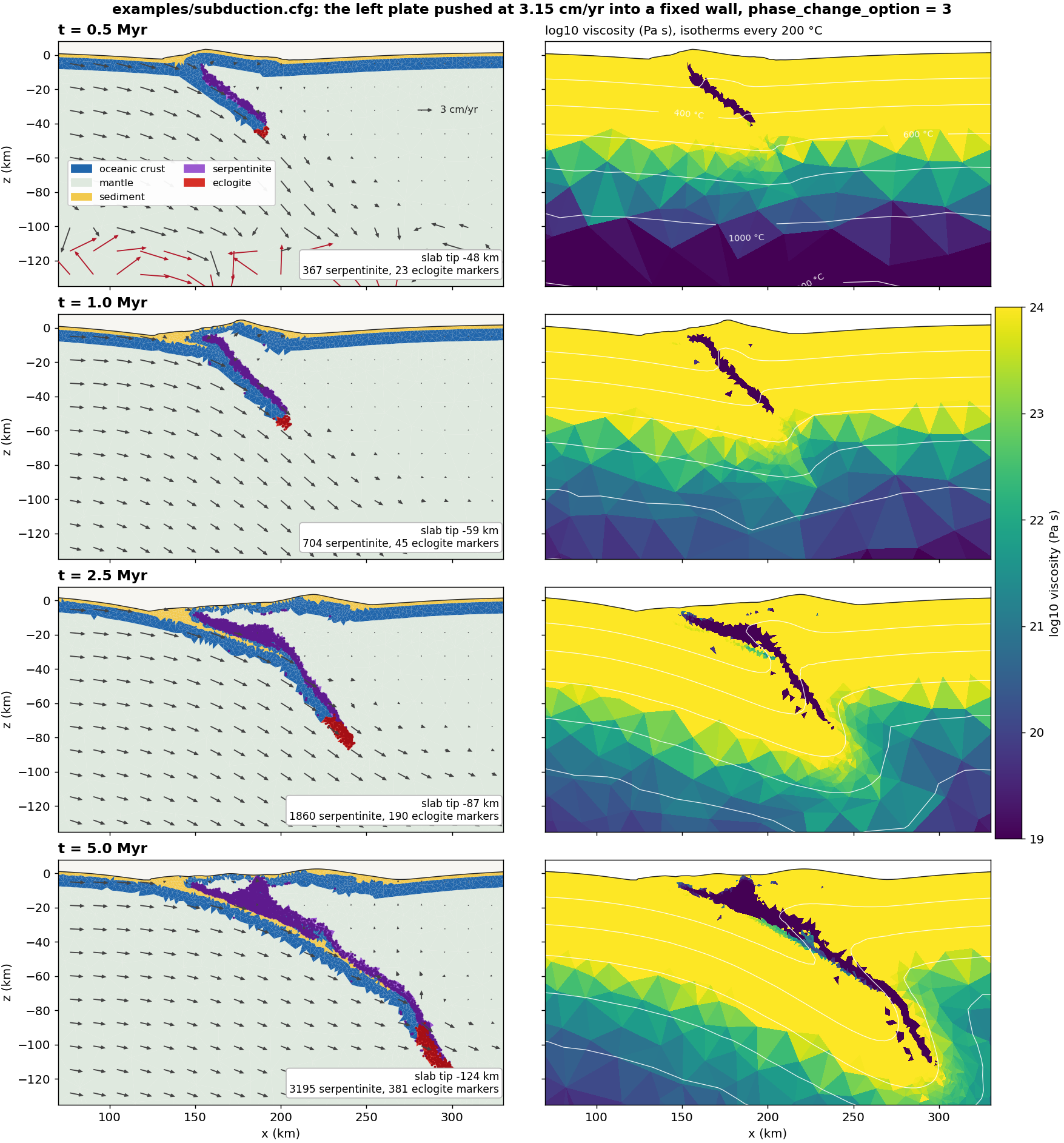
Things to look for as the run proceeds (the figure is the reference run):
- Serpentinite from the first frame. The slab is already in place, so mantle just above its top converts at once: about 370 markers by 0.5 Myr, 3200 by 5 Myr. On the viscosity panels this layer sits at the 10¹⁹ Pa s floor and is the weakest material in the model.
- Eclogite starts at the slab tip. A few dozen markers have converted by 0.5 Myr, where the tip sits near 50 km; the count grows to about 380 by 5 Myr, when the deepest 30 km of the slab is eclogite.
- The slab tip reaches 50 km at 0.5 Myr, 85 km at 2.5 Myr and about 125 km at 5 Myr, keeping a dip of 30–35° on its way down. The cold core stays at the 10²⁴ Pa s viscosity cap and drags the isotherms down with it.
- The wedge corner serpentinizes wholesale. The mantle between the
overriding plate's crust and the slab top lies within one grid cell of
crust, so by 2.5 Myr a body 20–25 km thick and 50 km long has converted.
This is the geometric rule at work, not a thermal one; Exercise 3 shows
how
serpentinization_thicknesscontrols it. - The trench fills with sediment and the overriding plate's crust bends down into it, while the incoming plate at the left wall keeps its three layers thanks to the restored wall.
How the mesh keeps up
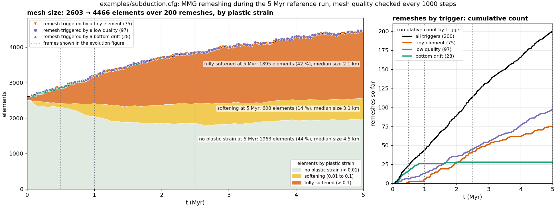
The mesh grows by two thirds over the run, and the left panel shows where
the new elements go. Elements with no plastic strain fall from 2500 to about
2000 as the deforming band widens into them, and they stay coarse at a
median of 4.5 km. Fully softened elements, those past pls1 = 0.1, grow from
none to about 1900, 42 % of the mesh, at a median size of 2.1 km against the
6 km resolution and the 1.5 km MMG floor. That is the MMG metric at work:
mmg_metric_refine_coeff shrinks the target size where plastic strain has
accumulated, along the plate interface and in the wedge, and nowhere else.
The 200 remeshes have three triggers, each checked every
quality_check_step_interval steps. A tiny element is one whose area has
dropped below smallest_size times the resolution squared. Low quality is
an element quality below min_quality, 0.2 here. Bottom drift is a bottom
node more than max_boundary_distortion times resolution, 6 km here, from
the 160 km base. The first two are the ordinary triggers and fire throughout.
Bottom drift belongs to the first million years, 26 of its 28 remeshes, while
the slab tip sinks through the lower mantle and the Winkler bottom adjusts;
after that it stops. Each remesh moves
the element count by only a few tens, because the conservative MMG mode
freezes elements that are not yielding, distorted or tiny. Remeshing takes
under 1 % of the wall time; the phase changes take 5 %.
Exercise 3: change the thickness of the serpentinite layer
serpentinization_thickness sets how far above the slab top mantle can
convert, counted in 3 km grid cells. It must be positive, so the zero case
is the rule switched off.
| Run | Thickness | Change | What you should see |
|---|---|---|---|
| None | 0 km | has_serpentinization = no | The interface locks. The slab tip falls behind from 2 Myr on and reaches only 100 km at 5 Myr, the slab necks and tears below the overriding plate, and both plates thicken and buckle: the trench reaches 9 km at 2.5 Myr, 3 km deeper than the reference |
| Reference | 5 km | serpentinization_thickness = 5e3 (one cell) | Steady subduction to 125 km at 5 Myr; trench deepens to 6.5 km by 3 Myr and recovers to 4 km; about 3200 serpentinite and 380 eclogite markers |
| Thick | 10 km | serpentinization_thickness = 10e3 (two cells) | Half again as much serpentinite (4600 markers) in a wedge body that reaches further down the slab; trench about 1 km shallower on average, with less swing; slab tip 120 km; a quarter fewer eclogite markers |
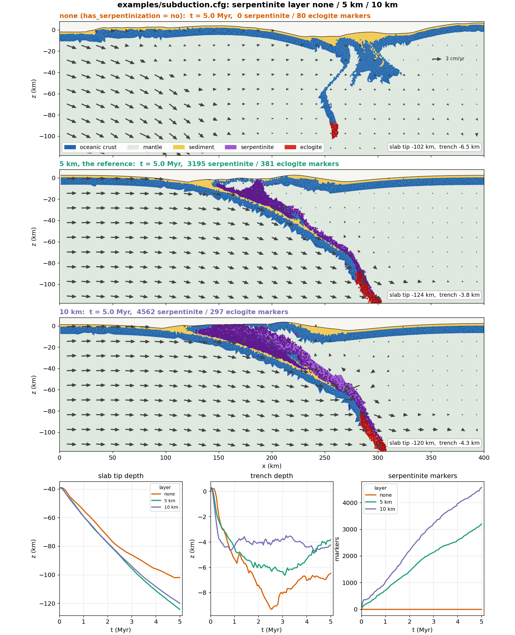
What the comparison shows:
- The weak layer is what makes this model subduct. Without it the sediment seed alone cannot keep the interface slipping; convergence goes into thickening and buckling the plates, the slab falls behind and tears below the overriding plate, and the velocity arrows show the whole overriding plate being pushed instead of the slab sliding under it. Such a run also works the mesh hard: the thickened plates load the Winkler bottom unevenly and most of its remeshes are bottom-drift triggers, and an earlier build of this case died in a remeshing failure at 3.45 Myr.
- A thicker layer lubricates more. With two cells the trench is shallower by about 1 km on average and swings less, the forearc high is lower, and the wedge-corner body is larger. The slab tip ends 4 km shallower.
- Eclogite responds indirectly. The 10 km run has about 300 eclogite markers at 5 Myr against 380 in the reference. The rule did not change; the thicker weak layer keeps the slab crust shallower and warmer where it would otherwise cross the reaction boundary.
- Time step and cost barely change: 5.7 to 5.9 million steps for the two subducting runs, about 22 minutes alone on 6 threads; the locked run takes 4.3 million steps and 17 minutes because its plates move more slowly.
The reference and the 10 km run were each made twice, on the pull request's
branch and on master after the merge, with the same configuration. The
pairs agree on everything above, but differ in detail: the 10 km trench ended
1 km shallower than the reference in one pair and 0.5 km deeper in the other,
and the eclogite deficit was 40 % in one and 22 % in the other. That is the
chaotic scatter of a remeshing model. Read differences of that size as
suggestive, and the locking of the 0 km case, which starts by 1 Myr and grows,
as robust.
Restart case: stop the convergence and see what carries on
A run can be continued from any checkpoint with changed settings. DES writes a
checkpoint every checkpoint_frame_interval frames, 10 by default, so the
reference run leaves its last one at frame 100, 5 Myr. The example is already
set up to restart from it; switch the restart on, give the run another two
million years and stop the push:
is_restarting = yes
restarting_from_modelname = model-subduction
restarting_from_frame = 100
max_time_in_yr = 7e6
vbc_val_x0 = 0                    # the left plate is held still
The restart runs in the same directory as the parent, reads its frame 100 and checkpoint, and writes frames 100 to 140 of its own; the extra two million years take about two minutes. The question it answers is which parts of the model were driven by the push and which carry on by themselves once convergence stops, as after a collision or a plate reorganisation.
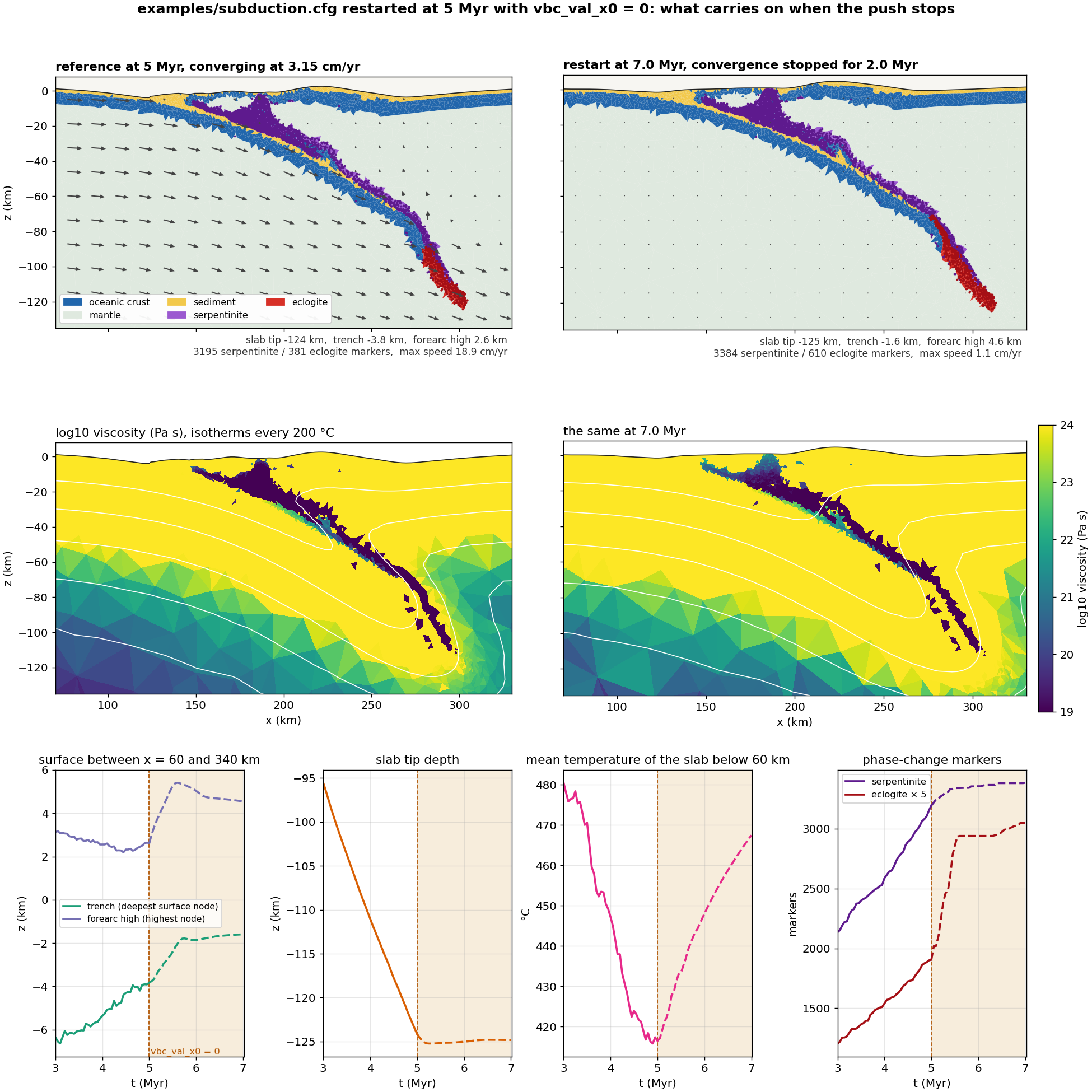
- The slab stops. Its tip sank 13 km per million years while pushed and less than 1 km in the two million years after. There is no slab pull to speak of here: the plate it hangs from is held at the wall, and sinking further would mean stretching a plate at the 10²⁴ Pa s viscosity cap. This model subducts because it is pushed. The peak speed in the domain falls from 19 to 1 cm/yr.
- The surface rebounds first, then smooths. Within the first million
years the trench shallows from 3.8 to 1.8 km and the forearc high rises from
2.6 to 5.3 km; the whole overriding plate between x = 100 and 300 km comes
up by 1.5 to 2.5 km. That is isostatic rebound: the shear on the plate
interface that was holding the overriding plate down is gone. After that
the levels hardly move, the high eases back to 4.6 km, and surface diffusion
takes over: at
surface_diffusivity = 5e-7it reaches √(κt) ≈ 6 km in two million years, enough to cut the root-mean-square slope between x = 60 and 340 km by a third while the overall relief stays near 6 km. Diffusion rounds the slopes; it does not remove the relief. The incoming plate next to the held wall sags by up to 6 km, a wall effect to be aware of. - The slab warms and reacts until it runs out of crust. Below 60 km the slab's mean temperature rises by 50 °C over the two million years, because nothing cold arrives any more. Eclogite is the one thing that speeds up: 381 markers at 5 Myr become 588 by 5.75 Myr as the stationary crust heats across the basalt–eclogite boundary and the eclogite front climbs from 87 to 71 km depth. Then it stops, at 610 markers by 7 Myr: the crust above 71 km is too shallow to cross the boundary however warm it gets, so a stationary slab saturates. Serpentinite grows by 190 markers in the first half million years, then stops too: its rule is geometric and needs new mantle to be brought over crust.
Two cautions. Pick a restart frame that is not a remesh step, since a checkpoint written on one is not bit-recoverable. And a restart is a new realization of a chaotic run, so compare it with the parent's trend, as the bottom row does, rather than with a single frame.
Change one parameter at a time, and keep a log of what you changed.
Troubleshooting
The rows marked "observed" come from runs made for this tutorial; the others are the usual causes.
| Symptom | Part | Cause and fix |
|---|---|---|
| Strain stays diffuse, no single fault | 1 | The band cannot be narrower than its elements: smallest_size too large (observed at 1, Exercise 2) or resolution too coarse. Or softening is too slow: pls1 large, or weakzone_plstrain below pls1 so the seed is not pre-softened |
| Fault dies and a new one forms | 1 | Slow softening or a thick layer favours several short-lived faults over one long-lived one; lower pls1 or thin the layer (Lavier, Buck & Poliakov 2000) |
| Time step shrinks and the run slows | both | dt follows the smallest element; the mesh has refined more than you want. Raise smallest_size or lower mmg_metric_refine_coeff (observed: 0.017 yr at the stock 0.01 against 0.11 yr at 1) |
Stops at input with a mattype_* message | 2 | Each active rule needs its source and target set to distinct, valid materials; check the mattype_* lines against num_materials |
Stops at input: serpentinization_thickness too small | 2 | It must be at least one grid cell, resolution × vt_size |
remeshing_option 13 refused | 2 | Restored side walls need an MMG build: make ndims=2 usemmg=1 |
| Serpentinite appears far from the slab | 2 | The rule has no temperature gate below 150 km; a slab bend can make a whole grid column crust-dominant. Set serpentinization_wet_crust_margin >= 0 to confine it |
| Slab stalls, plates thicken and buckle | 2 | The interface is too strong: this is the has_serpentinization = no case of Exercise 3. Check mattype_serpentinite is set and the sediment and serpentinite friction angles are low. Such a run also piles up bottom-drift remeshes and can end in [DES exit 41]; to carry it on, restart from the last checkpoint with max_boundary_distortion halved to 0.5 |
Next Steps
- Copy the example files to start your own model, rather than writing configs from scratch
- Add surface processes with GoSPL coupling
- Refine the mesh around faults with MMG
- Go to 3D with
oblique-rift-3d.cfgandconjugate-faults-3d.cfg; see Velocity boundary conditions (3D) and Weak zones
References
- Choi, E., Tan, E., Lavier, L. L. & Calo, V. M. (2013). DynEarthSol2D: an efficient unstructured finite element method to study long-term tectonic deformation. J. Geophys. Res. Solid Earth, 118, 2429–2444.
- Lavier, L. L., Buck, W. R. & Poliakov, A. N. B. (1999). Self-consistent rolling-hinge model for the evolution of large-offset low-angle normal faults. Geology, 27, 1127–1130.
- Lavier, L. L., Buck, W. R. & Poliakov, A. N. B. (2000). Factors controlling normal fault offset in an ideal brittle layer. J. Geophys. Res., 105, 23431–23442.
- Tan, E., Lavier, L. L., Van Avendonk, H. J. A. & Heuret, A. (2012). The role of frictional strength on plate coupling at the subduction interface. Geochem. Geophys. Geosyst., 13, Q10006.
- Hacker, B. R., Abers, G. A. & Peacock, S. M. (2003). Subduction factory 1: theoretical mineralogy, densities, seismic wave speeds, and H₂O contents. J. Geophys. Res., 108, 2029.
- Ulmer, P. & Trommsdorff, V. (1995). Serpentine stability to mantle depths and subduction-related magmatism. Science, 268, 858–861.
- Grove, T. L., Till, C. B., Lesher, E., Chatterjee, N., Médard, E. & Gaetani, G. A. (2009). The role of H₂O in subduction zone magmatism. Annu. Rev. Earth Planet. Sci., 37, 503–520.