Rate-and-state friction in a finite-width shear band

This tutorial uses two small 2D DynEarthSol models to follow slow loading, rapid slip and recovery. You will run a uniform velocity-weakening (VW) band, then compare it with a VW patch between velocity-strengthening (VS) flanks. Five figures connect the model inputs to its time histories and spatial response.

What is rate-and-state friction?

Rate-and-state friction describes resistance that depends on sliding rate and a state variable, θ, which evolves with the deformation history. The parameters a and b control the frictional response: at steady sliding, a−b > 0 is velocity strengthening and a−b < 0 is velocity weakening. Velocity weakening can promote instability; the surrounding stiffness, loading and state evolution also matter.

Here frictional deformation occupies a 2 km thick band, rather than an infinitely thin fault. Our displacement measure is the horizontal displacement of the upper band interface minus that of the lower interface. It includes elastic deformation as well as localized inelastic deformation.

By the end, you should be able to connect a slip-speed peak to displacement accumulation, stress release and a reduction in the solver time step, and explain why the VS flanks creep while the central VW patch accumulates a displacement deficit and then catches up.

Prerequisites

Download and extract the workshop files. They contain Tutorial.ipynb, a browser-readable Tutorial.html, model inputs, reference outputs and the data behind the five figures.

Use Linux, macOS or Windows Subsystem for Linux (WSL). On Windows, run both DES and Jupyter inside WSL. You need a C++ compiler, Make, Boost.Program_options, HDF5 and Python 3.10 or later. HDF5 development headers and libraries are required: this tutorial reads VTKHDF spatial fields, so keep hdf5=1 when building DES. Installing Python's h5py alone does not provide the system development package needed to compile DES.

Install the dependencies for your operating system before building.

Ubuntu 22.04 or later (including Ubuntu in WSL):

sudo apt update
sudo apt install -y git g++ make libboost-program-options-dev libhdf5-dev pkg-config python3 python3-venv

macOS: install the Xcode Command Line Tools (xcode-select --install, if not already installed) and Homebrew, then run:

brew install boost libomp hdf5 pkg-config python

libomp supplies the OpenMP runtime for Apple's compiler. The pinned DES revision below automatically locates HDF5 on Ubuntu and macOS; do not pass Ubuntu-specific HDF5_INCLUDE_DIR or HDF5_LIB_DIR paths on macOS.

Build and check DES

This exercise was checked against the public DES revision 1b4e94f1c333fdade9dc512cf9cb20e10e8e9aad. Use a separate checkout so an existing working copy is preserved.

git clone --recursive https://github.com/GeoFLAC/DynEarthSol.git DynEarthSol-tutorial
cd DynEarthSol-tutorial
git checkout 1b4e94f1c333fdade9dc512cf9cb20e10e8e9aad
git submodule update --init --recursive
make config ndims=2 opt=2 openmp=1 hdf5=1
make -j2 ndims=2 opt=2 openmp=1 hdf5=1
export DYNEXE="$PWD/dynearthsol2d"
export OMP_NUM_THREADS=1
export OMP_DYNAMIC=FALSE
"$DYNEXE" --help

Check that make config reports hdf5 1 and existing HDF5 include and library directories for your installation. The same build commands work on Ubuntu and macOS. Check that the help lists rsf_slip_rate_projection_option, rsf_dtheta_max and use_global_velocity_scaling. The executable must be a 2D HDF5 build. Keep this terminal open so DYNEXE remains defined. The mesh is small enough that one OpenMP thread is appropriate.

Only if HDF5 auto-detection fails: first install the HDF5 development package listed above. If it is installed but the build still cannot find it, check its location and rerun the complete build command with explicit paths. These overrides select an existing installation; they do not install HDF5.

On Ubuntu x86_64, the serial development package normally uses the paths below. Verify them before building; other architectures can use a different library directory.

ls /usr/include/hdf5/serial/H5Lpublic.h
ls /usr/lib/x86_64-linux-gnu/hdf5/serial/libhdf5.so
make -j2 ndims=2 opt=2 openmp=1 hdf5=1 \
  HDF5_INCLUDE_DIR=/usr/include/hdf5/serial \
  HDF5_LIB_DIR=/usr/lib/x86_64-linux-gnu/hdf5/serial

On macOS with Homebrew, use the installed formula's prefix:

ls "$(brew --prefix hdf5)/include/H5Lpublic.h"
ls "$(brew --prefix hdf5)/lib/libhdf5.dylib"
make -j2 ndims=2 opt=2 openmp=1 hdf5=1 \
  HDF5_INCLUDE_DIR="$(brew --prefix hdf5)/include" \
  HDF5_LIB_DIR="$(brew --prefix hdf5)/lib"

Each multi-line make block is one shell command: the trailing backslashes continue it onto the next line. Keep the path assignments on that command; do not run them as separate commands after make. Once the build succeeds, continue with the DYNEXE exports and help check above.

Prepare Python

Change to the extracted DES-RSF-Tutorial directory, then run:

export TUTORIAL_DIR="$PWD"
python3 -m venv .venv
source .venv/bin/activate
python -m pip install -r resources/requirements.txt
python -m jupyterlab

Open Tutorial.ipynb and a JupyterLab terminal (File → New → Terminal). Run each example's bash block in that terminal; run its python block as a notebook cell. In the terminal, run these three commands once before Example 1, replacing the executable path with the absolute path from the build step:

export DYNEXE="/absolute/path/to/DynEarthSol-tutorial/dynearthsol2d"
export OMP_NUM_THREADS=1
export OMP_DYNAMIC=FALSE

A JupyterLab terminal normally inherits these variables if they were exported before JupyterLab started. Repeating the commands makes the run settings explicit. Keep this terminal for both examples; repeat the three commands if you open a new terminal.

To study the results without running DES, use the supplied reference paths in the notebook's setup cell. The reference figures and numerical data are included in the download; no solver is needed for that route.

How the model works

The model is 100 km wide and 10 km deep. A horizontal band lies between depths of 4 and 6 km. The upper boundary moves in the positive x direction at 10⁻⁹ m/s and has zero vertical velocity; the bottom is fixed. The side boundaries do not impose a velocity. Both examples use the same geometry and loading.

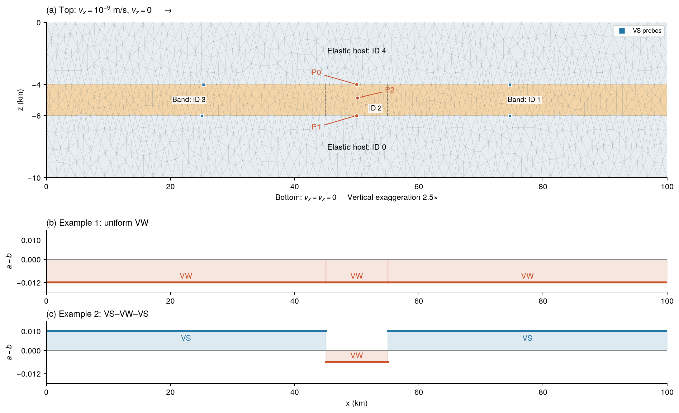
Figure 1. (a) Model geometry, boundary loading and monitor positions; depth is exaggerated by 2.5×. P0 and P1 sample the upper and lower faces of the band near x = 50 km, and P2 samples its interior. (b) Spatial distribution of a−b in Example 1: the entire band is VW. (c) Spatial distribution of a−b in Example 2: a central VW patch lies between VS flanks.

Setting	Value
Domain / band thickness	100 × 10 km / 2 km
Central patch	x = 45–55 km
Density / bulk modulus / shear modulus	2700 kg/m³ / 50 GPa / 30 GPa
Band cohesion / characteristic distance	4 MPa / 0.005 m
Reference and loading velocity	10⁻⁹ m/s
Nominal mesh resolution	400 m
Model duration	850 years

Geometry, material IDs and friction

decollement.poly defines 14 vertices, 18 segments and five material regions. The band order from left to right is 3–2–1, while arrays in [mat] are indexed by material ID 0,1,2,3,4. The lower and upper hosts are IDs 0 and 4. Their very large cohesion keeps them elastic in this exercise.

Case / region	Material ID	a	b	a−b
Example 1: entire band	1, 2, 3	0.003	0.015	−0.012
Example 2: left VS	3	0.011	0.001	+0.010
Example 2: central VW	2	0.011	0.017	−0.006
Example 2: right VS	1	0.011	0.001	+0.010

Both examples use state_var_model=1 and the same characteristic distance. The two cfg files already contain these assignments. The .poly vertices at (50, −4) and (50, −6) km let P0/P1 match the interface at x = 50 km; they do not introduce another material division. The annotated resources/POLY_GUIDE.md in the download explains the point, segment and region blocks.

What is measured?

P0 and P1 provide the signed across-band horizontal speed vx(P0) − vx(P1). Figures 2–3 show its absolute value, |vx(P0) − vx(P1)|. Across-band displacement is calculated from the P0 and P1 horizontal coordinates as [x(P0,t) − x(P1,t)] − [x(P0,t_initial) − x(P1,t_initial)], where t_initial is the first saved monitor sample. This retains the sign of displacement; integrating the absolute speed would instead accumulate travel in both directions. P2 provides local shear stress and θ.

Figure 5 instead interpolates displacement along both band interfaces at the same initial x positions. This lets the spatial profiles and the VS/VW time histories use exactly the same quantity.

Quick start: run Example 1

Step 1: prepare and inspect the inputs

Start in the extracted tutorial directory. Use a fresh run-directory name when repeating a calculation; mkdir below deliberately stops if it already exists.

export TUTORIAL_DIR="$PWD"
mkdir -p "$TUTORIAL_DIR/results"
export RUN_DIR="$TUTORIAL_DIR/results/example1"
mkdir "$RUN_DIR" && mkdir "$RUN_DIR/output" && \
  cp resources/models/example1_uniform_vw.cfg resources/models/decollement.poly "$RUN_DIR/"
sed -n '/^\[mat\]/,/^\[monitor\]/p' "$RUN_DIR/example1_uniform_vw.cfg"

In [sim], max_time_in_yr=850 is physical model time. output_time_interval_in_yr=25 sets the normal field-save interval to 25 model years; output_step_interval=1000000 also requests a save after that many solver steps. earthquake_output_step_interval=1000 requests more frequent fields during a detected rapid episode. In [monitor], step_interval=10 saves monitor points every ten solver steps. These are output intervals, not the solver's physical time step.

Step 2: run DES and inspect its output

cd "$RUN_DIR"
"$DYNEXE" example1_uniform_vw.cfg

Wait for the solver to finish successfully. Confirm the startup log reports one OpenMP thread. Then inspect the files:

head -n 2 output/monitor_point_0.csv
head -n 2 output/monitor_point_1.csv
head -n 2 output/monitor_point_2.csv
ls output/model.save.*.vtkhdf | head
printf 'Example 1 output: %s\n' "$RUN_DIR"

CSV coordinates and displacement use metres, velocities m/s, times seconds and stresses Pa. Compare the requested query_x/query_z with the selected coord_x/coord_z: P0/P1 should match x = 50000 m exactly, while P2 can use a nearby interior mesh node. VTKHDF save files contain spatial fields; chkpt files are restart checkpoints.

Step 3: load the results in the notebook

The notebook starts in the tutorial directory, independently of the terminal's current directory. Set RUN to your Example 1 output and SECOND to the Example 2 directory you will create below. For the no-solver route, uncomment the two reference assignments.

from pathlib import Path
import sys
import numpy as np
import h5py
import matplotlib.pyplot as plt

ROOT = Path.cwd().resolve()
assert (ROOT / "resources/tutorial_tools.py").is_file(), "Open the notebook in the tutorial directory."
sys.path.insert(0, str(ROOT / "resources"))
import tutorial_tools as tt

RUN = ROOT / "results/example1"
SECOND = ROOT / "results/example2"
# RUN = ROOT / "resources/reference/example1_uniform_vw"
# SECOND = ROOT / "resources/reference/example2_vs_vw_vs"
FIGURES = ROOT / "resources/figures"
print(f"Example 1 analysis source: {RUN}")
print(f"Example 2 analysis source: {SECOND}")

# Read monitor CSVs: P0-P1 relative horizontal velocity/displacement,
# plus P2 shear stress, state variable and friction histories.
history = tt.band_history(RUN)
# Find |vx(P0) - vx(P1)| >= 1e-3 m/s (1 mm/s).
# Group exceedances separated by at most 86400 s (one model day).
events = tt.find_events(history)
for number, event in enumerate(events, start=1):
    print(f"Event {number}: {event['start_yr']:.3f} yr; "
          f"peak speed {event['peak_relative_speed']:.3f} m/s")

start_yr is the first saved threshold-exceeding time in each group; peak_relative_speed is its largest sampled absolute relative speed. This is an analysis criterion, separate from DES's internal rapid-output trigger, not a physical definition of an earthquake. It measures motion at P0/P1, not every slipping region in the model, and can miss peaks between saved samples. The defaults are threshold=1e-3 and merge_gap_s=86400; the plotting helpers below use those same defaults internally.

The five numbered figures below are supplied reference figures. The plotting cells create additional figures from the directories selected by RUN and SECOND; selecting reference paths deliberately plots the supplied runs. The basic workshop saves fewer spatial fields than the figure-generation runs, so compare physical trends and actual saved times before expecting a matching image. Python plotting is provided; the exercises focus on interpreting and comparing results.

The supplied Example 1 has two detected episodes, near 648.255 and 836.241 years. Here an episode groups crossings of an across-band speed of 10⁻³ m/s; this analysis threshold is distinct from DES's automatic output trigger.

Worked example 1: from loading to rapid slip

Read the full history

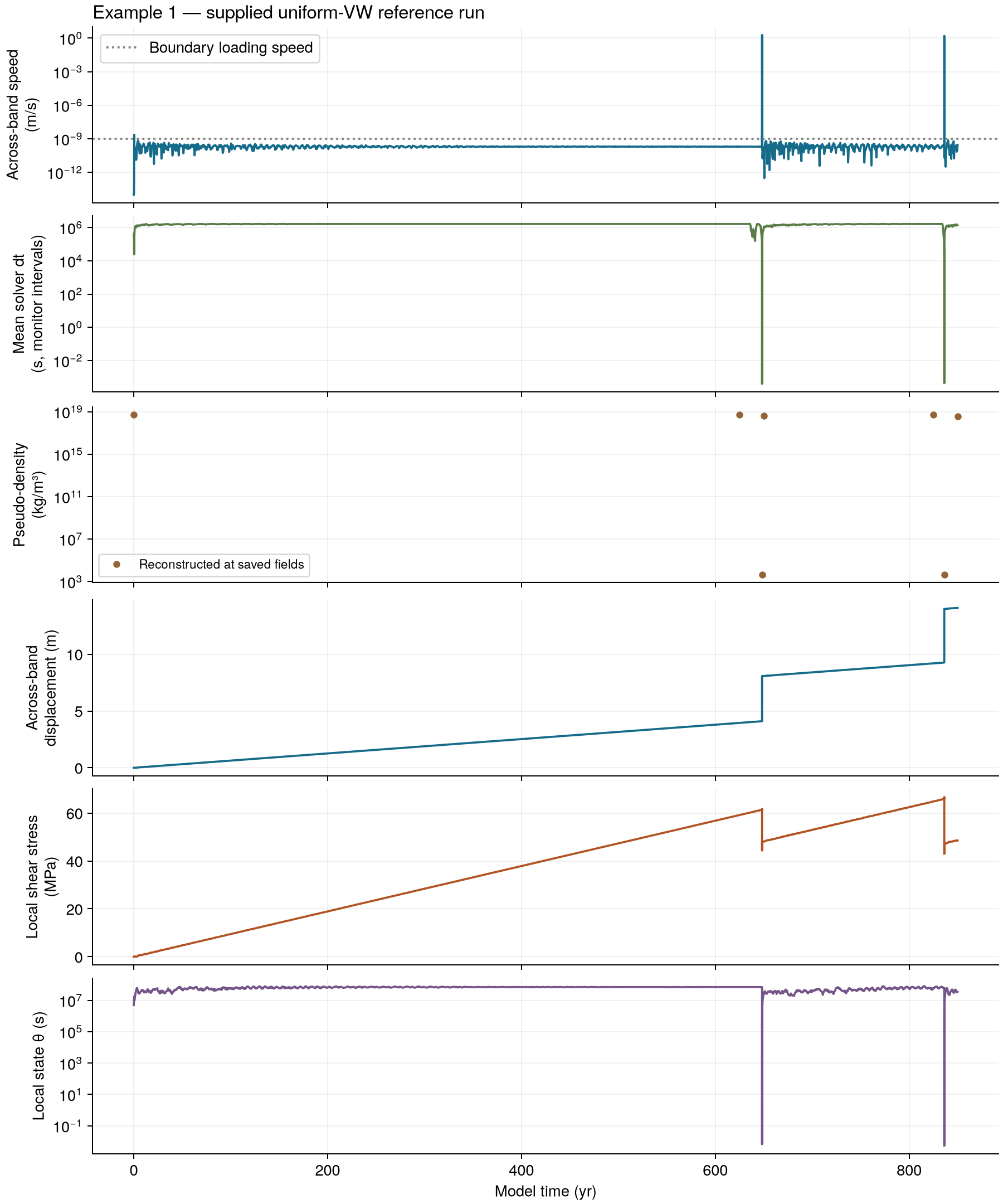
Figure 2. Six panels from the supplied Example 1 reference run. Read vertically at each event: speed rises, mean solver dt shrinks, reconstructed pseudo-density decreases, displacement increases abruptly, and shear stress drops. Stress then reloads. The dt curve uses monitor-interval averages; pseudo-density markers use the seven supplied spatial fields. Markers are not joined because they do not resolve the evolution between field saves.

Plot the same six panels from RUN on a shared model-time axis: speed, mean solver time step, pseudo-density, displacement, stress and state. plot_history calculates the mean time step as diff(time_s) / diff(step) between consecutive monitor records and plots it at each interval's midpoint. The workshop records every 10 solver steps, so this is an interval average, not an individual step's dt. It resolves the time-step trend more densely than the spatial field saves, but can smooth short-lived extrema. Both the supplied Figure 2 and your plot use this same monitor-based calculation.

The pseudo-density panel represents numerical inertia from mass scaling, not physical rock density. pseudo_density_samples reads the run's cfg and instantaneous VTKHDF fields and reconstructs the pinned solver's formula: rho_pseudo = K / min(S * Vmax, sqrt(M / rho))**2, where S is inertial_scaling, Vmax is the largest magnitude of an element's mean nodal velocity (floored by the prescribed boundary-speed bound), and M is the shear modulus by default, or the bulk modulus for mass_scaling_reference_speed=bulk. The helper requires uniform elastic moduli and physical density, as in these workshop models.

With the workshop's default shear-speed ceiling, K=50 GPa, G=30 GPa and rho=2700 kg/m³, pseudo-density cannot fall below rho*K/G=4500 kg/m³. The VTKHDF density array contains physical density, not this quantity. Reconstruction from a saved velocity field is a diagnostic, not a direct record of assembled nodal masses or their exact update times. Sparse field saves can miss rapid changes; mean dt alone cannot determine pseudo-density because other constraints, including the RSF state limit, also control dt.

# Plot speed, mean dt, reconstructed pseudo-density, displacement, stress and theta.
fig = tt.plot_history(history, title=f"Example 1 — {RUN.name}")
plt.show()

Rebuild the supplied Figure 2 (PNG/PDF) and its numerical CSV data with python resources/plot_history_figure.py from the extracted tutorial directory. It uses the bundled reference run; your notebook uses RUN. The available field saves can differ, so compare actual sample times and physical trends.

Follow one complete event

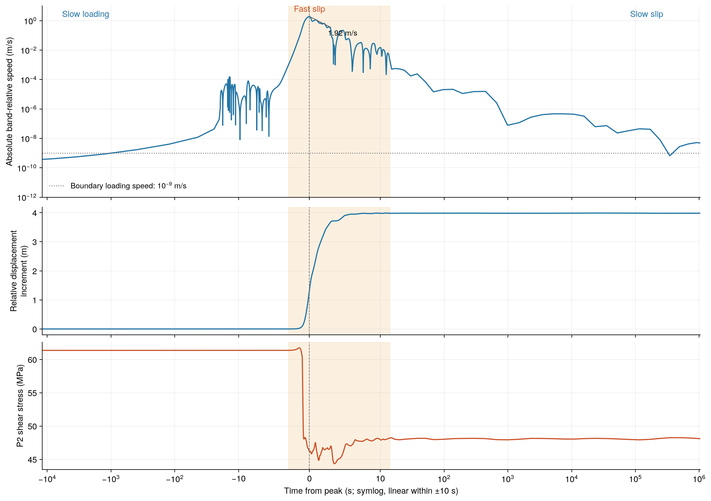
Figure 3. Time is measured from the sampled speed peak. The continuous symlog axis is linear within ±10 s and logarithmic outside, so both slow tails and the rapid interval remain visible. Shading spans the first to last 10⁻³ m/s threshold exceedance in this episode.

The sampled peak reaches approximately 1.92 m/s. Most displacement accumulates while the band moves rapidly and stress is released; the recovery continues well beyond the rapid interval. Equal distances along this time axis are not equal durations.

EVENT_INDEX = 0  # Set to 1 for the second detected episode.
assert EVENT_INDEX < len(events), "No such detected episode; inspect the full history first."
event = events[EVENT_INDEX]
time_from_peak = history["time_s"] - event["peak_time_s"]
print(f"Sampled peak speed: {event['peak_relative_speed']:.3f} m/s")
print(f"Threshold-crossing envelope: {event['span_s']:.3f} s")
print(f"Local stress drop to the low-rate recovery sample: "
      f"{event['local_shear_stress_drop_mpa']:.2f} MPa")

Plot the selected episode from RUN. This helper shows a short window around the threshold-crossing interval on a linear time axis; Figure 3 uses a longer symlog window to show loading and recovery. The displacement here is zero at the first threshold-crossing sample.

# Plot the selected event from 10 s before its first exceedance to 10 s
# after its last; time zero is the sampled speed peak (default detection).
fig_event = tt.plot_event(history, event_index=EVENT_INDEX)
fig_event.suptitle(f"Example 1 — {RUN.name}; event {EVENT_INDEX + 1}")
plt.show()

Exercise 1. Identify the loading, rapid-slip and recovery intervals in Figures 2–3 and the rapid-slip interval in your plotted event. Then set EVENT_INDEX=1 and rerun the event cells to compare the second episode. Two episodes give one observed interval, not a recurrence distribution.

Worked example 2: a VW patch between VS flanks

Change the frictional contrast

The second cfg changes the band friction values while preserving geometry, loading, cohesion and characteristic distance. The relevant arrays are:

direct_a = [0.003, 0.011, 0.011, 0.011, 0.003]
evolution_b = [0.015, 0.001, 0.017, 0.001, 0.015]

The centre is VW and the flanks are VS. Do not overwrite Example 1's cfg. Return to the tutorial directory in the same terminal and run the second case:

cd "$TUTORIAL_DIR"
export SECOND_DIR="$TUTORIAL_DIR/results/example2"
mkdir "$SECOND_DIR" && mkdir "$SECOND_DIR/output" && \
  cp resources/models/example2_vs_vw_vs.cfg resources/models/decollement.poly "$SECOND_DIR/"
cd "$SECOND_DIR"
"$DYNEXE" example2_vs_vw_vs.cfg

After successful completion, return to the notebook:

# Read Example 2 monitors and apply the same speed/gap criteria as Example 1.
second_history = tt.band_history(SECOND)
second_events = tt.find_events(second_history)
for number, event in enumerate(second_events, start=1):
    print(f"Event {number}: {event['start_yr']:.3f} yr; "
          f"peak speed {event['peak_relative_speed']:.3f} m/s")

Plot Example 2's monitor history from SECOND before examining its spatial response. Compare the event timing and displacement jumps with Example 1.

# Use the same six panels, including mean dt and pseudo-density, for Example 2.
fig_second = tt.plot_history(second_history, title=f"Example 2 — {SECOND.name}")
plt.show()

Inspect the spatial response during rapid slip

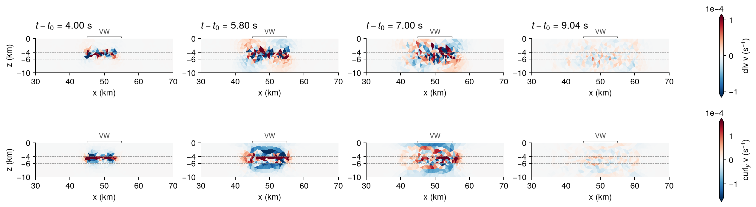
Figure 4. Top: divergence of velocity. Bottom: its out-of-plane curl. Times are seconds after the first event's analysis threshold crossing. The bracket marks the central VW interval. The full band is visible, with values beyond each fixed colour range saturated.

In the 2D x–z plane, these scalar diagnostics are div v = ∂vx/∂x + ∂vz/∂z and curl_y v = ∂vx/∂z − ∂vz/∂x, both in s⁻¹. They highlight dilatational and rotational motion around the slipping band. Derivatives are calculated directly within each linear triangular element on the current mesh, without smoothing.

View the velocity-gradient animation. Its frames have nonuniform physical time intervals; read their timestamps rather than interpreting playback speed as physical time.

This calculation retains adaptive mass scaling and damping. The gradients show the spatial mechanical response, but do not by themselves establish physical P/S wave speeds or isolate pure wave amplitudes. Large gradients inside the band also include its localized deformation.

The next cell reads the supplied Figure 4 data. Its results refer to the reference wavefield calculation, independently of SECOND.

print("Source: supplied Figure 4 wavefield data")
with np.load(FIGURES / "04_wavefield_data.npz") as data:
    offsets = data["time_after_detection_s"].copy()
    divergence = data["divergence"].copy()
    curl_y = data["curl_y"].copy()
index = int(np.argmin(abs(offsets - 5.8)))
print(f"Field time after detection: {offsets[index]:.3f} s")
print(f"Maximum absolute divergence: {np.max(abs(divergence[index])):.3e} 1/s")
print(f"Maximum absolute curl_y: {np.max(abs(curl_y[index])):.3e} 1/s")

To inspect your own spatial fields, the following cell uses SECOND and selects saved fields before, near the peak of, and after its first event. The upper row shows signed plastic-strain increments from the pre-event field; the lower row shows instantaneous nodal speed. These diagnostics complement the divergence/curl reference figure. Read the actual saved times printed below: a sparse save may miss the speed peak. This plot needs pre-event and recovered fields; if an input variation has no detected or recovered event, inspect its full history first.

plot_snapshots chooses the last pre-event field whose maximum nodal speed is below 1e-7 m/s, the field nearest the sampled speed peak, and the first field at or after the first post-event P0/P1 relative-speed sample below 1e-7 m/s. Here "recovered" denotes that speed threshold, not proof that the band has physically locked; inspect the printed snapshot times.

SPATIAL_EVENT_INDEX = 0
assert SPATIAL_EVENT_INDEX < len(second_events), "No such detected spatial episode."
# Select saved fields before, nearest the sampled peak, and after recovery;
# plot plastic-strain changes from the pre-event field and nodal speed.
fig_spatial, selected_fields = tt.plot_snapshots(
    SECOND, second_history, event_index=SPATIAL_EVENT_INDEX)
fig_spatial.suptitle(f"Example 2 — {SECOND.name}; event {SPATIAL_EVENT_INDEX + 1}")
for label, row in selected_fields:
    print(f"{label}: {row['time_s'] / tt.YEAR:.6f} yr; step {row['step']}")
plt.show()

Exercise 2. Compare the four snapshots and the animation. Where are the largest gradients? How does the host response change as the slip accelerates and decays? Distinguish evidence for spatial motion from a measurement of a wave's propagation speed.

Compare creep and sudden displacement

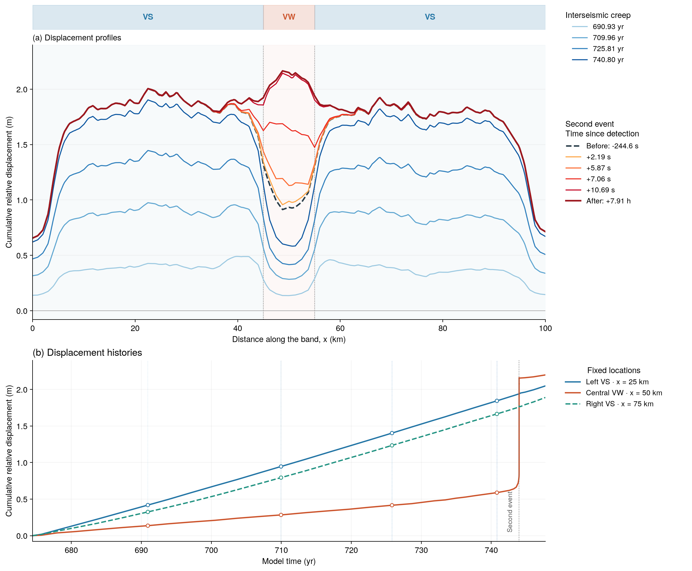
Figure 5. Top strip: positions of the VS flanks and central VW patch. Upper plot: cumulative across-band horizontal displacement versus x at successive saved times. Blue curves show interseismic accumulation; warm colours resolve the second rapid episode. Lower plot: time histories of the same displacement at x = 25 km (left VS), 50 km (central VW) and 75 km (right VS). Circles and dotted lines identify the interseismic snapshots shown above.

All curves use the same zero at 674.465 years, after the first event. VS flanks accumulate displacement steadily while the VW centre falls behind. Near 743.974 years, the centre makes a rapid displacement jump and catches up. The finite band still deforms between events: “locked” here means a relative displacement deficit, not exactly zero motion.

Explore the supplied data behind this figure. These arrays belong to the illustrated reference run, regardless of the paths selected for your own runs.

print("Source: supplied Figure 5 displacement data")
with np.load(FIGURES / "05_displacement_histories.npz") as data:
    positions = data["x_km"].copy()
    sample_times = data["time_s"].copy()
    displacements = data["displacement_m"].copy()
index = int(np.argmin(abs(sample_times / tt.YEAR - 740.8)))
print(f"At {sample_times[index] / tt.YEAR:.3f} yr:")
for x, displacement in zip(positions, displacements[index]):
    print(f"  x = {x:.0f} km: {displacement:.3f} m")

Now plot displacement profiles and VS/VW histories from SECOND using the same interface interpolation as the reference analysis. If a quiet field is available between the first event's recovery and the second event, start from the earliest such field to reveal the next loading interval and displacement jump. Otherwise, start from the earliest saved field in the run. All curves use that one common reference time, shown in the title. Markers represent saved fields, and straight connecting lines do not resolve unsaved rapid motion. The reference Figure 5 uses a post-first-event origin and dense saves around its second event; your reference time depends on the fields actually available.

# List VTKHDF save files with their saved model times and solver steps.
catalog = sorted(tt.field_catalog(SECOND), key=lambda row: row["time_s"])
if len(second_events) >= 2:
    recovered_time = second_history["time_s"][second_events[0]["quiet_index"]]
    next_start = second_history["time_s"][second_events[1]["start_index"]]
    quiet_fields = [row for row in catalog if recovered_time <= row["time_s"] < next_start]
    if quiet_fields:
        catalog = [row for row in catalog if row["time_s"] >= quiet_fields[0]["time_s"]]
x_km = np.linspace(0, 100, 401)
profiles = []
base_field = None
for row in catalog:
    # Read mesh, velocity, plastic strain, material IDs and stress from VTKHDF.
    field = tt.read_field(row["path"])
    if base_field is None:
        base_field = field
    assert np.array_equal(field["connectivity"], base_field["connectivity"]), "Mesh topology changed."
    assert np.array_equal(field["material"], base_field["material"]), "Material IDs changed."
    # Interpolate upper-minus-lower horizontal displacement at common initial x.
    profiles.append(tt._interface_profile(field, x_km))
profiles = np.asarray(profiles)
profiles -= profiles[0].copy()
field_times_yr = np.asarray([row["time_s"] / tt.YEAR for row in catalog])
positions_km = np.asarray([25., 50., 75.])
position_histories = np.asarray([np.interp(positions_km, x_km, profile)
                                 for profile in profiles])

fig_comparison, axes = plt.subplots(2, 1, figsize=(10, 8), layout="constrained")
# Limit the legend to six profiles; the histories use every saved field.
indices = np.unique(np.linspace(0, len(catalog) - 1, min(6, len(catalog)), dtype=int))
for index in indices:
    axes[0].plot(x_km, profiles[index], label=f"{field_times_yr[index]:.3f} yr")
for left, right, name in [(0, 45, "VS"), (45, 55, "VW"), (55, 100, "VS")]:
    axes[0].axvspan(left, right, color="0.5", alpha=.06 if name == "VS" else .15)
    axes[0].text((left + right) / 200, .96, name, transform=axes[0].transAxes,
                 ha="center", va="top")
for column, label in enumerate(["Left VS (25 km)", "Central VW (50 km)", "Right VS (75 km)"]):
    axes[1].plot(field_times_yr, position_histories[:, column], ".-", label=label)
axes[0].set(xlabel="Initial x (km)", ylabel="Across-band displacement (m)")
axes[1].set(xlabel="Model time (yr)", ylabel="Across-band displacement (m)")
for ax in axes:
    ax.grid(alpha=.18)
    ax.legend(fontsize=9)
fig_comparison.suptitle(f"Example 2 — {SECOND.name}; common zero at {field_times_yr[0]:.3f} yr")
plt.show()

To save a generated figure as PNG and PDF, run, for example, tt.save_figure(fig_comparison, "example2_selected_run_displacement"). Files are written under results/figures/; using the same name again replaces those exported figures. The supplied numbered figures remain available for comparison. For denser profiles and histories, run figure5_dense.cfg in a fresh directory, set SECOND to that directory and rerun the Example 2 cells.

Exercise 3. Explain how the central displacement deficit in the upper panel corresponds to the lower panel's slowly rising VW curve. Compare the VW jump with the VS increments across the same event. Why would three curves with separate arbitrary displacement offsets obscure this comparison?

Try a controlled variation

Copy Example 2 into a new run directory and change only the central material's evolution_b entry. Keep track of its a−b value and compare displacement histories, maximum speed and local stress release. Do not assume that every VW configuration must produce an earthquake, or that changing friction leaves the event timing unchanged.

For denser observations with unchanged physical parameters, the download also includes figure2_dense.cfg, figure5_dense.cfg and figure4_wave.cfg. Copy one together with decollement.poly into a fresh directory containing output/ and pass its filename to DES, just as above. The first two run for 850 years; the wavefield case stops at 700 years and saves fields every ten steps. It can produce hundreds of megabytes of output. These are the observation settings used to prepare the figures; data and figures are already supplied for the workshop.

Troubleshooting

Symptom	Check
HDF5 headers or library not found during the build	Install libhdf5-dev on Ubuntu or hdf5 with Homebrew on macOS, remove old explicit HDF5 path overrides, and rerun the build with hdf5=1. Python's h5py is not a substitute for these build dependencies.
omp.h or libomp not found on macOS	Run brew install libomp, then rerun the build.
Executable not found	Set DYNEXE to the absolute path of the compatible 2D executable, then check test -x "$DYNEXE".
Unknown RSF option	Check the solver revision and --help; an older generic DES build may lack these controls.
.poly file not found	Run inside the case directory containing both the cfg and decollement.poly.
No VTKHDF fields	Confirm an HDF5-enabled build and successful completion; look under the run's output/.
Missing results in a notebook cell	Correct RUN/SECOND, or deliberately select the supplied reference paths.
Very slow execution on a small mesh	Set OMP_NUM_THREADS=1 and OMP_DYNAMIC=FALSE before starting DES.
Event snapshots differ from a published figure	Check the cfg's output cadence and actual stored times; the basic workshop uses fewer field saves.

Next steps

Use the supplied .poly guide to change the central patch width, or compare both detected events without changing the inputs. Keep each run separate and record one change at a time.

For the broader context, see the DES documentation and Lapusta et al. (2000).