Groundwater heat transport: Ogata–Banks
Steady groundwater carries heat from a hot inlet along a saturated column while conduction spreads the front.
Largest temperature error: 1.306% of the imposed 1 K jump, over all nodes and five saved times; the pressure stays exactly steady.
| Dimension | 3D |
| Build | make ndims=3 from the poromechanics source (not yet merged; DynEarthSol #134) |
| Inputs | heat.zip |
| Reproduce with | DynEarthSol 3774df0 |
Problem setup
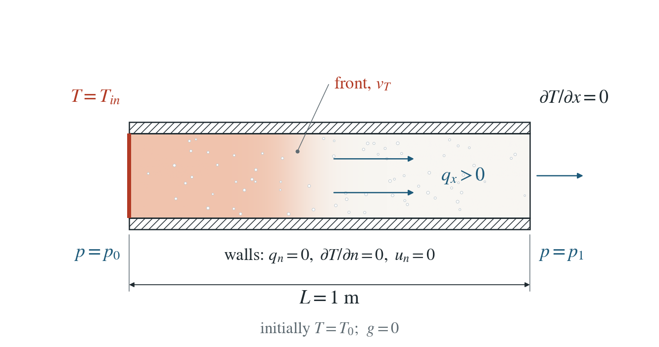
Steady groundwater flow. Pa, m²/(Pa s), m/s; gravity zero. Pressure is prescribed at both ends.
Temperature and mechanical conditions. Initially K. At the left end is set to K. Sides and right end have zero conductive heat flux; heat can advect out. Normal motion is fixed on every face.
Reference regime. Constant properties and steady Darcy flux; fixed mesh, no mechanical pressure feedback. Deliberately scaled coefficients isolate transport; this is not an aquifer application.
Input and how to run
Every file this example needs is in heat.zip. Run from that folder:
# Runs the 3D column (1 m long, 2×2 elements across) for 8192 steps to 0.47 s and writes column.save.* and column.chkpt.* every 2048 steps, with column.info listing the five frames.
dynearthsol3d input.cfg
Settings that define this example
| Setting | Value | What it does here |
|---|---|---|
control.has_fluid_thermal_advection | true | turns on heat transport by the Darcy flux, with the combined rock–water heat capacity |
bc.hbc_x0 | 2 | type 2: pressure prescribed at the inlet end |
bc.hbc_x1 | 2 | type 2: pressure prescribed at the outlet end |
bc.hbc_pressure | [2,1,0,0,0,0] | 2 Pa at x = 0 and 1 Pa at x = 1 m: a steady pressure drop that drives q_x = 1 m/s |
ic.pore_pressure_option | 1 | 1: start from the linear pressure profile between the two prescribed ends, so the flow is steady from the start |
bc.tbc_x0 | 1 | 1: fixed temperature at the inlet |
bc.tbc_val_x0 | 274.15 | inlet temperature T_in = T_0 + 1 K |
bc.tbc_z1 | 0 | 0: the top is insulated, like the other sides and the outlet |
ic.temp_background | 273.15 | initial temperature T_0 = 273.15 K |
mat.hydraulic_perm | [1] | 1 m², with fluid_visc = 1 Pa s: mobility κ/μ = 1 m²/(Pa s) |
mat.fluid_bulk_modulus | [1e-6] | deliberately tiny, which makes the hydraulic storage large without changing the steady flux |
mat.therm_cond | [23500.0] | λ chosen with the capacities to give thermal diffusivity D = 0.005 m²/s |
mat.heat_capacity | [2000.0] | solid specific heat; with rho0, porosity and fluid_heat_capacity it sets the bulk capacity C = 4.7 MJ/(m³ K) |
mat.fluid_heat_capacity | [4000.0] | water specific heat; ρ_f c_f q_x / C sets the front speed v_T |
input.cfg holds all 60 settings that differ from DES’s defaults; dynearthsol3d -h lists every option with its default.
Output
See Running the examples for output files, the Python reader and ParaView conversion.
| Field | What to look at |
|---|---|
temperature | nodal temperature, normalized as (T − T_0)/(T_in − T_0) and plotted along the column |
pore pressure | checked to stay on the steady linear profile at every saved time |
Result: DES and the analytical solution
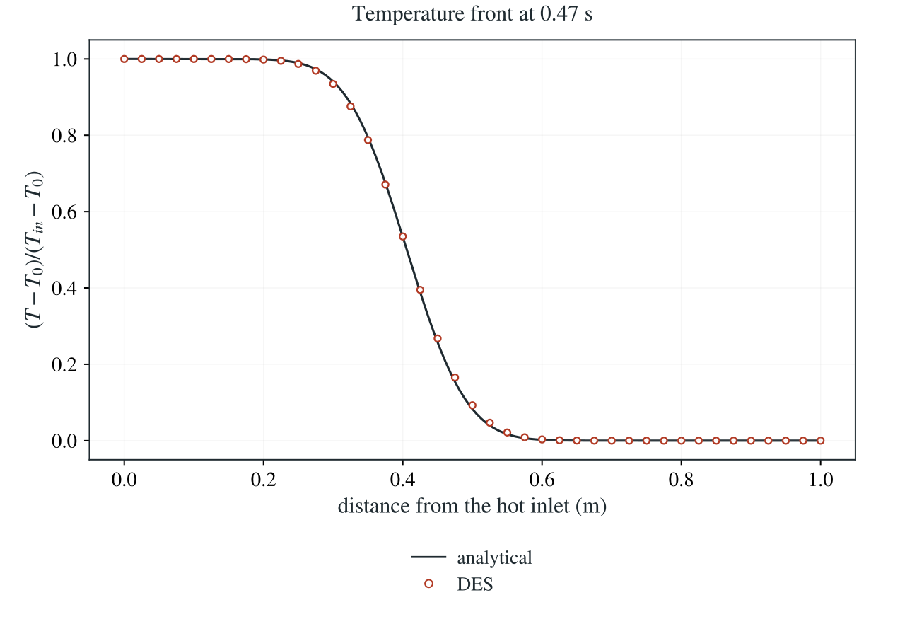
Normalized temperature along the column at the last saved time: line, the Ogata–Banks solution moving at the bulk-capacity speed v_T; symbols, DES nodes (about 40 shown).
This checks Darcy heat advection and the mixed solid–fluid heat capacity: the front moves at the bulk-capacity speed, not the pore-water velocity. It does not test enthalpy conservation with evolving storage.
To reproduce the whole study behind this figure, from the DES source folder:
python3 tests/functional/hydromechanics/check_heat_transport.py dynearthsol3d OUT/3d --spacings 0.0125 0.00625 0.003125 --steps 8192 --restart
python3 tests/functional/hydromechanics/check_heat_transport.py dynearthsol2d OUT/2d --spacings 0.025 0.0125 0.00625 0.003125 --steps 8192 --restart
python3 tests/functional/hydromechanics/check_heat_transport.py dynearthsol2d OUT/2d-steps --spacings 0.0125 --steps 512 1024 2048 4096 --restart
The study’s full numbers: record.json.
Analytical reference
is bulk volumetric heat capacity, and fluid and solid specific heat capacities, thermal conductivity and Darcy flux. Here , , and ; the final front position is .
Derivation
For constant C and divergence-free steady flux, the bulk sensible-heat balance reduces to the equation above. Dividing by C shows that the thermal front travels at vT, rather than at qx or qx/φ.
Laplace-transform the normalized equation in time with its zero initial condition. Reject the growing spatial root and impose the unit step at x = 0. Inverting this transform gives the two complementary-error-function terms above.
Ogata and Banks (1961), USGS Professional Paper 411-A; the transport solution is applied here to normalized temperature. Evaluated stably using erfcx in check_heat_transport.py.
Validity and limits
The analytical solution is semi-infinite: , for and . The numerical domain ends at m with zero conductive flux, so the comparison uses early times before the front reaches that boundary. Constant-capacity, divergence-free flow is tested; general evolving-storage enthalpy conservation is not established. The intentionally tiny fluid modulus makes the hydraulic storage large without changing the steady flux.